Python Monte Carlo Simulation in Excel

In our data-dominated monetary setting, Monte Carlo simulation is a key software for danger modeling and quantitative methods. Whereas many people will proceed to make use of Excel as our most popular platform, it’s unlucky that Excel’s base capabilities require the additional work that many monetary professionals might want to full for any stochastic modeling. On this information, we’ll present you how one can ‘plug’ a Monte Carlo simulation in Python into Excel to develop a hybrid optimization for superior danger evaluation and monetary modeling. 

Understanding Monte Carlo Simulation in Danger Administration

Monte Carlo simulation works by operating 1000’s or hundreds of thousands of random realizations, with the preliminary enter variables outlined by likelihood distributions. The probabilistic modeling strategy provides a number of advantages in conditions of unsure outcomes and monetary danger administration.

The methodology defines likelihood distributions for unsure variables, generates random variates, performs calculations for every realization, and assesses statistical outcomes. Monte Carlo simulation provides insights past deterministic fashions, proving particularly helpful in portfolio optimization and credit score danger modeling.

Danger metrics resembling Worth-at-Danger (VaR), Anticipated Shortfall, and likelihood of loss will be estimated with Monte Carlo estimation. Monte Carlo strategies present analysts with most flexibility to mannequin complicated correlations throughout variables, use non-normal distributions, and account for time-dependent parameters according to reside market situations.

Python Libraries for Monte Carlo Danger Modeling

Many Python libraries present excellent assist for Monte Carlo simulation and statistical evaluation: 

1. NumPy: NumPy is the spine as a result of its highly effective array operations and random quantity technology. It performs vectorized operations, enabling environment friendly large-scale simulations. The library additionally offers many statistical capabilities for likelihood distributions in monetary modeling.
2. SciPy: SciPy builds on NumPy with statistical distributions and optimization algorithms. It provides over 80 distributions and exams for danger modeling. SciPy additionally helps complicated finance functions by way of numerical integration strategies.
3. Pandas: Pandas is extremely helpful for information manipulation and time sequence evaluation. Its dataframe integrates easily with Excel by way of numerous import and export capabilities, making monetary information evaluation and aggregation simple.
4. Matplotlib and Seaborn: Matplotlib and Seaborn allow professional-quality information visualizations of simulation outcomes. These visualizations can embrace danger distributions or sensitivity analyses, which will be embedded into Excel reviews.

Excel Integration Methods: Python-Excel Connectivity

There are a number of fashionable Excel Python integration choices, and so they have totally different strengths for Monte Carlo danger modeling:

1. xlwings is probably the most seamless integration choice. This library allows bidirectional communication between Excel and Python, supporting reside information trade and real-time simulation outcomes.
2. openpyxl and xlsxwriter each present a fantastic file-based integration choice to make use of if a direct connection isn’t wanted. This library allows creating complicated reviews, dealing with a number of worksheets, formatting, and charts in Excel from Python simulations. Both library can do the job.
3. COM automation with pywin32 permits for deep integration of Excel on Home windows machines, because the library automates the creation and manipulation of Excel objects, ranges, and charts. This feature could also be helpful if you wish to create subtle danger dashboards and interactive modeling environments.

Fingers-On Implementation: Constructing a Monte Carlo Danger Mannequin

It’s time to create a sturdy portfolio danger evaluation system utilizing Excel and a Python Monte Carlo simulation. Utilizing this sensible instance, we’ll show inventory worth forecasting, correlation evaluation, and the computation of danger metrics.

1. Arrange the Python setting and put together the information.

import numpy as np
import pandas as pd
import matplotlib.pyplot as plt
from scipy import stats
from datetime import datetime, timedelta
import warnings
warnings.filterwarnings('ignore')

# Portfolio configuration
shares = ['AAPL', 'GOOGL', 'MSFT', 'AMZN', 'TSLA']
initial_portfolio_value = 1_000_000
time_horizon = 252
num_simulations = 10000

np.random.seed(42)
annual_returns = np.array([0.15, 0.12, 0.14, 0.18, 0.25])
annual_volatilities = np.array([0.25, 0.22, 0.24, 0.28, 0.35])
portfolio_weights = np.array([0.25, 0.20, 0.25, 0.15, 0.15])

correlation_matrix = np.array([
    [1.00, 0.65, 0.72, 0.58, 0.45],
    [0.65, 1.00, 0.68, 0.62, 0.38],
    [0.72, 0.68, 1.00, 0.55, 0.42],
    [0.58, 0.62, 0.55, 1.00, 0.48],
    [0.45, 0.38, 0.42, 0.48, 1.00]
])

2. Monte Carlo Simulation Engine

def monte_carlo_portfolio_simulation(returns, volatilities, correlation_matrix,
                                     weights, initial_value, time_horizon, num_sims):
    # Convert annual parameters to every day
    daily_returns = returns / 252
    daily_volatilities = volatilities / np.sqrt(252)

    # Generate correlated random returns
    L = np.linalg.cholesky(correlation_matrix)

    # Storage for simulation outcomes
    portfolio_values = np.zeros((num_sims, time_horizon + 1))
    portfolio_values[:, 0] = initial_value

    # Run Monte Carlo simulation
    for sim in vary(num_sims):
        random_shocks = np.random.regular(0, 1, (time_horizon, len(shares)))
        correlated_shocks = random_shocks @ L.T

        daily_asset_returns = daily_returns + daily_volatilities * correlated_shocks
        portfolio_daily_returns = np.sum(daily_asset_returns * weights, axis=1)

        for day in vary(time_horizon):
            portfolio_values[sim, day + 1] = portfolio_values[sim, day] * (1 + portfolio_daily_returns[day])

    return portfolio_values

# Execute simulation
print("Operating Monte Carlo simulation...")
simulation_results = monte_carlo_portfolio_simulation(
    annual_returns, annual_volatilities, correlation_matrix,
    portfolio_weights, initial_portfolio_value, time_horizon, num_simulations
)

3. Danger Metrics Calculation and Evaluation

def calculate_risk_metrics(portfolio_values, confidence_levels=[0.95, 0.99]):
    final_values = portfolio_values[:, -1]
    returns = (final_values - portfolio_values[:, 0]) / portfolio_values[:, 0]
    losses = -returns

    mean_return = np.imply(returns)
    volatility = np.std(returns)

    # VaR
    var_metrics = {}
    for confidence in confidence_levels:
        var_metrics[f'VaR_{int(confidence*100)}%'] = np.percentile(losses, confidence * 100)

    # Anticipated Shortfall
    es_metrics = {}
    for confidence in confidence_levels:
        threshold = np.percentile(losses, confidence * 100)
        es_metrics[f'ES_{int(confidence*100)}%'] = np.imply(losses[losses >= threshold])

    max_loss = np.max(losses)
    prob_loss = np.imply(returns  0 else 0

    return {
        'mean_return': mean_return,
        'volatility': volatility,
        'sharpe_ratio': sharpe_ratio,
        'max_loss': max_loss,
        'prob_loss': prob_loss,
        **var_metrics,
        **es_metrics
    }

risk_metrics = calculate_risk_metrics(simulation_results)

4. Excel Integration and Dashboard Creation

def create_excel_risk_dashboard(simulation_results, risk_metrics, shares, weights):
    portfolio_data = pd.DataFrame({
        "Inventory": shares,
        "Weight": weights,
        "Anticipated Return": annual_returns,
        "Volatility": annual_volatilities
    })

    metrics_df = pd.DataFrame(record(risk_metrics.gadgets()), columns=['Metric', 'Value'])
    metrics_df['Value'] = metrics_df['Value'].spherical(4)

    final_values = simulation_results[:, -1]
    # Excel export code would comply with right here

summary_stats = {
    "Preliminary Portfolio Worth": f"${initial_portfolio_value:,.0f}",
    "Imply Ultimate Worth": f"${np.imply(final_values):,.0f}",
    "Median Ultimate Worth": f"${np.median(final_values):,.0f}",
    "Customary Deviation": f"${np.std(final_values):,.0f}",
    "Minimal Worth": f"${np.min(final_values):,.0f}",
    "Most Worth": f"${np.max(final_values):,.0f}"
}

summary_df = pd.DataFrame(record(summary_stats.gadgets()), columns=['Statistic', 'Value'])

plt.determine(figsize=(10, 6))
plt.hist(final_values, bins=50, alpha=0.7, shade="skyblue", edgecolor="black")

plt.axvline(initial_portfolio_value, shade="purple", linestyle="--",
            label=f'Preliminary Worth: ${initial_portfolio_value:,.0f}')
plt.axvline(np.imply(final_values), shade="inexperienced", linestyle="--",
            label=f'Imply Ultimate Worth: ${np.imply(final_values):,.0f}')

var_95 = initial_portfolio_value * (1 - risk_metrics['VaR_95%'])
plt.axvline(var_95, shade="orange", linestyle="--",
            label=f'95% VaR: ${var_95:,.0f}')

plt.title("Portfolio Worth Distribution - Monte Carlo Simulation")
plt.xlabel("Portfolio Worth ($)")
plt.ylabel("Frequency")
plt.legend()
plt.grid(True, alpha=0.3)
plt.savefig("portfolio_distribution.png", dpi=300, bbox_inches="tight")
plt.shut()

5. Superior State of affairs Evaluation

def scenario_stress_testing(base_returns, base_volatilities,             correlation_matrix, weights, initial_value, eventualities):
    scenario_results = {}
    for scenario_name, (return_shock, vol_shock) in eventualities.gadgets():
        stressed_returns = base_returns + return_shock
        stressed_volatilities = base_volatilities * (1 + vol_shock)

        scenario_sim = monte_carlo_portfolio_simulation(
            stressed_returns, stressed_volatilities, correlation_matrix,
            weights, initial_value, time_horizon, 5000
        )

        scenario_metrics = calculate_risk_metrics(scenario_sim)
        scenario_results[scenario_name] = scenario_metrics

    return scenario_results


stress_scenarios = {
    "Base Case": (0.0, 0.0),
    "Market Crash": (-0.20, 0.5),
    "Bear Market": (-0.10, 0.3),
    "Excessive Volatility": (0.0, 0.8),
    "Recession": (-0.15, 0.4)
}

scenario_results = scenario_stress_testing(
    annual_returns, annual_volatilities, correlation_matrix,
    portfolio_weights, initial_portfolio_value, stress_scenarios
)

scenario_df = pd.DataFrame(scenario_results).T.spherical(4)

OUTPUT:

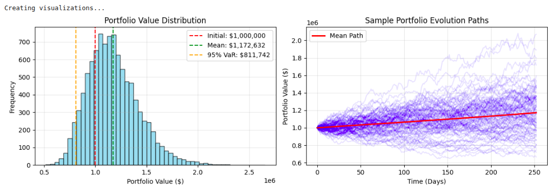
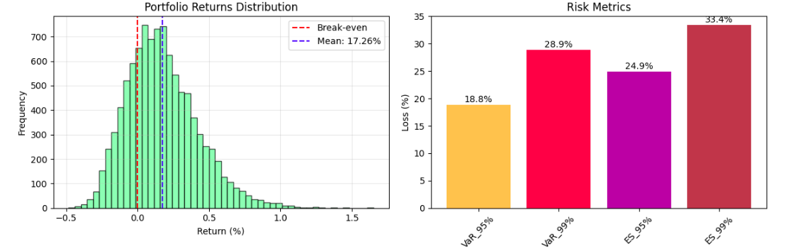
Output Evaluation:

The Monte Carlo-type simulation outputs present a complete understanding of danger evaluation by way of key statistics and visualizations of potential portfolio conduct in uncertainty. The Worth-at-Danger (VaR) methodologies sometimes point out for a diversified portfolio a 5% probability of experiencing greater than a 15-20% drop in worth over a 1-year time horizon. The Anticipated Shortfall metrics state the typical losses of unhealthy outcomes. The histogram of the portfolio worth distribution provides the probabilistic vary of outcomes, typically demonstrating a proper skewness sample with respect to danger on the draw back being concentrated, whereas the upside potential stays. 

Danger-adjusted efficiency statistics, such because the Sharpe ratio (normally measured within the vary of 0.8 to 1.5 for portfolios with balanced publicity), can point out if the potential anticipated return justifies the volatility publicity. The visualization of simulation paths signifies that market uncertainty is compounded over time, with particular person eventualities diverging distant from the imply trajectory, and the directional adjustments that happen over time present potential perception into strategic asset allocation or danger administration choices.

Superior Strategies: Enhancing Monte Carlo Danger Fashions

By using variance discount strategies, effectivity and accuracy in Monte Carlo simulations will be considerably improved. 

• Antithetic variates, management variates, and significance sampling strategies scale back the required variety of simulations to succeed in the extent of precision that’s desired.
• Quasi-Monte Carlo strategies are based mostly upon low-discrepancy sequences resembling `Sobol` or `Halton repeats, which is able to typically converge sooner than pseudo-random strategies, particularly for high-dimensional by-product pricing and portfolio optimization issues. 
• Copula-based dependency modeling capabilities use extra subtle correlation constructions than easy linear correlation. `Clayton`, `Gumbel`, and `t-copulas` all can match tail dependencies and asymmetries amongst belongings to offer lifelike estimates of `danger`. 
• Leap diffusion processes and regime-switching fashions to account for sudden shocks to the market and altering volatility regimes are one thing pure geometric Brownian movement can not mannequin. The prolonged strategies will contribute considerably to enhancing stress testing and tail danger evaluation.

Learn extra: A Information to Monte Carlo Simulation

Conclusion

Utilizing Python Monte Carlo simulation alongside Excel represents a serious advance in quantitative danger administration. This hybridized model successfully makes use of the computational rigor of Python coupled with the usability of Excel, leading to superior danger modeling instruments that retain usability enhancement together with performance. This implies monetary professionals can carry out superior situation evaluation, stress testing, and portfolio optimization whereas capitalizing on the familiarity of the Excel platform. The methodologies included on this tutorial present a paradigm on the way to assemble enterprise-wide danger administration programs, the place each analytical rigor and value can meet the identical vacation spot. 

In an ever-evolving regulatory and sophisticated market setting, the improved capability for adaptation and development of danger fashions will turn out to be ever extra related. Integrating Python-Excel permits us to attain the flexibleness and technical capabilities to shoulder these challenges whereas enhancing the transparency and auditability of danger administration mannequin growth. 

Continuously Requested Questions

Knowledge Science Trainee at Analytics Vidhya
I’m at present working as a Knowledge Science Trainee at Analytics Vidhya, the place I deal with constructing data-driven options and making use of AI/ML strategies to unravel real-world enterprise issues. My work permits me to discover superior analytics, machine studying, and AI functions that empower organizations to make smarter, evidence-based choices.
With a robust basis in pc science, software program growth, and information analytics, I’m keen about leveraging AI to create impactful, scalable options that bridge the hole between know-how and enterprise.
📩 You may as well attain out to me at [email protected]