
Amongst all of the instruments {that a} knowledge scientist has, it’s troublesome to search out one which has acquired a status as an efficient and reliable device like XGBoost. It was even talked about within the successful resolution of machine studying competitions on a website resembling Kaggle, which you will have in all probability visited. This isn’t by chance. The XGBoost algorithm is a champion with regard to efficiency on structured knowledge. This tutorial is the beginning of what you could learn about XGBoost, and it dissects its performance and follows a real-life XGBoost Python tutorial.
We’re going to see what’s so particular within the implementation of this gradient boosting. We’re additionally going to look at an XGBoost vs. Random Forest comparability to see the place it matches within the ensemble mannequin world. On the finish, you should have a transparent understanding of how you can apply this wonderful algorithm to your individual tasks.
What’s XGBoost and Why Ought to You Use It?
Primarily, XGBoost, the title of which is shortened from eXtreme Gradient Boosting, is an ensemble studying method. Think about it because the creation of a crew of specialised workers somewhat than relying on a generalist. It makes use of quite a few easy fashions, typically choice timber, to type a single very correct and strong predictive mannequin. The errors made by every new tree it provides to the crew trigger the corresponding mannequin to enhance with every new addition.
Why XGBoost?
So why then is XGBoost so widespread? The reply is its record of strengths that’s so spectacular.
- Distinctive Efficiency: It all the time offers the best high quality outcomes, significantly in tabular knowledge, which is normally current in enterprise issues.
- Velocity and Effectivity: The library is a well-oiled machine. It employs strategies resembling parallel processing to study fashions in a short while, even when working with enormous quantities of information.
- Inbuilt Checks and Balances: A typical side of machine studying is overfitting, whereby the mannequin learns too properly the coaching knowledge and is unable to work on new knowledge. XGBoost has regularization strategies that function a security web to preclude this.
- Offers with Sloppy Knowledge: Knowledge in the true world isn’t best. XGBoost has an inbuilt functionality to deal with lacking values and can prevent the tedious preprocessing section.
- Versatility: XGBoost is ready to work on each a classification downside (resembling fraud detection) and a regression process (resembling home worth prediction).
In fact, no device is ideal. The XGBoost energy is related to elevated complexity. It isn’t as clear as a easy linear mannequin, however it’s undoubtedly much less of a black field than a deep neural community. A single experiment found that XGBoost supplied a minor accuracy profit over logistic regression (98% frequent sense over 97%). It is because it wanted ten instances as a lot time to consider and make clear. You will need to know when that further improve in efficiency is well worth the effort of substituting.
Additionally Learn: Prime 10 Machine Studying Algorithms in 2026
How Boosting Works: A Crew of Learners
As a way to totally recognize the XGBoost, it’s worthwhile to have some idea of boosting. It’s one other philosophy, versus different ensemble strategies resembling bagging, that’s utilized by the random forests.
Suppose you’re introduced with two strategies for fixing a sophisticated downside with the assistance of a bunch of individuals.
- Bagging (The Committee Strategy): You award an issue to 100 people, get all of them to work individually, after which majority vote on the ultimate resolution. That is the best way Random Forest works. It constructs quite a few timber on the assorted random samples of the information and averages the votes.
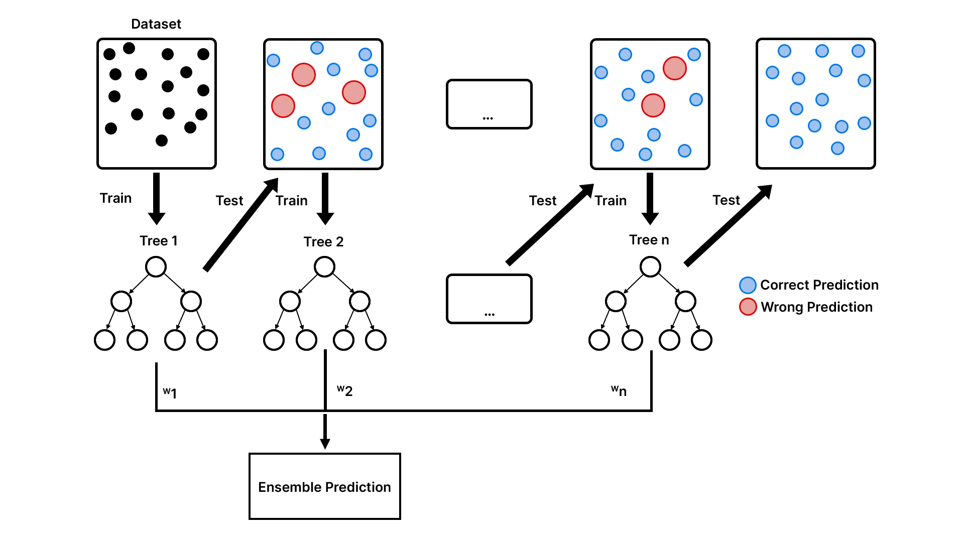
- Boosting (The Relay Race Strategy): You hand the issue over to the preliminary particular person. They work out a decision however commit some errors. The second individual, then, will solely have a look at the errors and try and rectify them. The third individual corrects the errors of the second individual and so forth.
XGBoost is predicated on the relay race technique. At a time, the brand new choice timber are involved with the information factors that the outdated timber missed. Technically, each new tree has been skilled to forecast the errors (often known as residuals) of the prevailing ensemble. The crew turns into resilient because it turns into extra exact as time passes, and the inclusion of a mannequin rectifies previous errors. It’s the magic of gradient boosting, which is carried out in a sequential and error-correcting approach.
All of the timber of the method are weak learners, easy shallow timber, which can or might not be any higher than guessing. Nevertheless, when tons of or hundreds of those poor learners are put collectively in a series, the ensuing mannequin is a powerhouse and a really particular predictor.
How XGBoost Builds Smarter, Extra Correct Timber
Choice timber are the basic constructing blocks; due to this fact, the best way that XGBoost expands them has a serious affect on its efficiency. Opposite to different algorithms, which fill out timber with a single department after which study the opposite, XGBoost builds a tree at every stage. The given technique normally offers a better-balanced tree, and optimization turns into simpler.
XGBoost will get its gradient element as a result of method through which splits are chosen. At each step, the algorithm considers the diploma to which a potential break up can lower the entire error of the mannequin and chooses the break up that provides probably the most helpful approach. It is because of this error-sensitive course of that XGBoost can successfully study extremely intricate patterns.
As a way to decrease overfitting, XGBoost defaults to protecting timber comparatively shallow and makes use of a studying charge, additionally known as shrinkage. Within the studying charge, the enter of each new tree is diminished, which forces the mannequin to get higher with time. The smaller the training charges are typically, the extra probably the timber are to create generalisation to the unseen knowledge.
How XGBoost Controls Velocity, Scale, and {Hardware} Effectivity
The parameter of XGBoost additionally allows you to regulate the event of timber with the assistance of the tree-method parameter. The only possibility is the histogram-based possibility, hist, which discretizes characteristic values and constructs timber based mostly upon the discretized characteristic values. That is quick and resource-efficient by way of CPU coaching. On very giant knowledge units, one can use an alternate approximate method, approx, however that is much less regularly utilized in present workflows. In circumstances the place a suitable GPU exists, gpuhist makes use of the identical histogram technique on the GPU and might assist in coaching time by a large margin.
hist is, in most cases, a robust default. Coaching velocity is essential, and GPU_hist ought to be used when GPU acceleration is current, and reserve ought to be used when specialised large-scale experiments are required.
XGBoost vs. Random Forest vs. Logistic Regression
It’s also a good suggestion to match XGBoost to the remainder of the favored fashions.
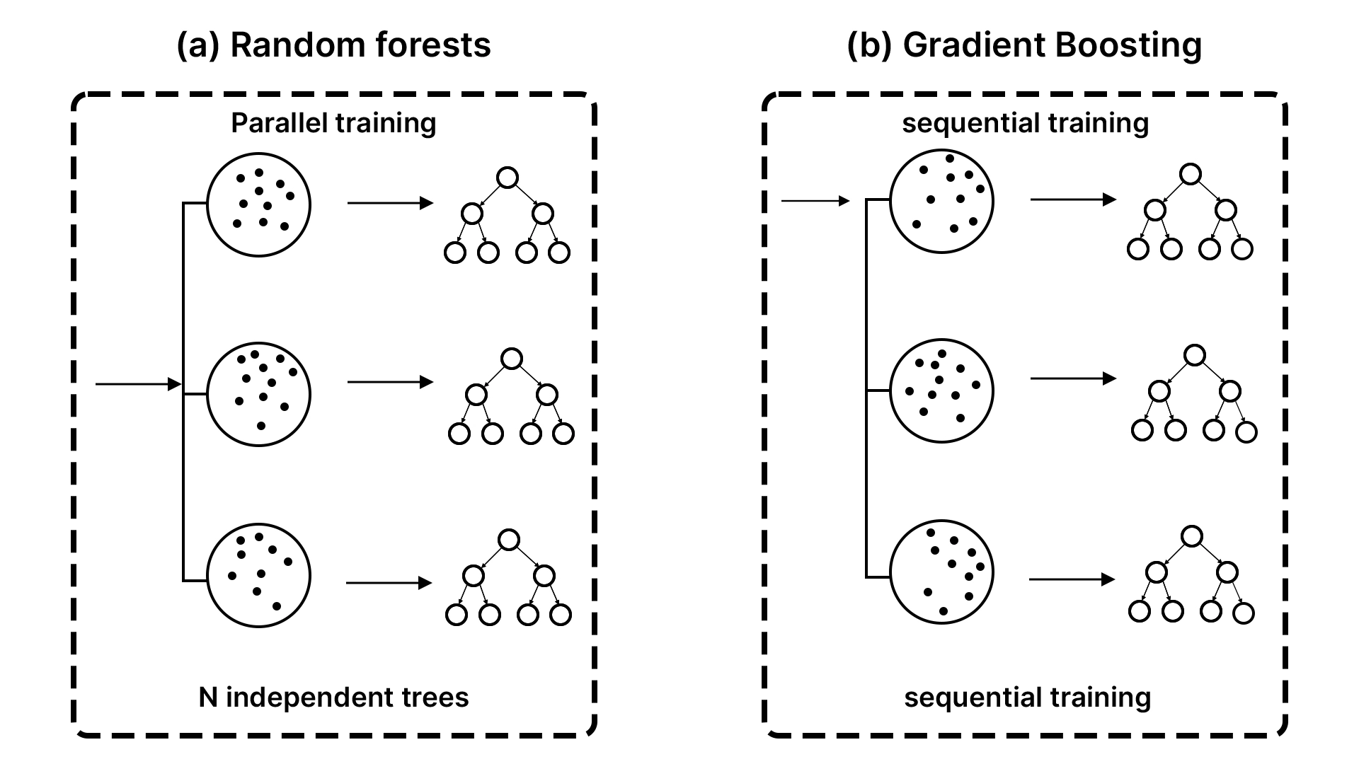
- XGBoost vs. Random Forest (The Relay Race vs. The Committee): XGBoost can be delicate to the sequence through which the timber are constructed, as we mentioned, thus it’s also extra proper in some conditions when it’s tuned accordingly. Random Forest produces unbiased and parallel timber, that suggest that it is vitally steady and fewer liable to overfitting. XGBoost performs higher than the choices in most conditions the place the optimum efficiency is required, and parameters may be set. Random Forest can be a fairly good mannequin for use in case you want a steady and highly effective mannequin that requires minimal efforts.
- XGBoost vs. Logistic Regression (The Energy Instrument vs. The Swiss Military Knife): Logistic Regression is an easy but quick and fairly simple to interpret linear mannequin. It’s used to mark courses in a straight line. It’s miraculously working and may be defined simply relying on its verdicts within the scenario the place your knowledge is linearly separable. The XGBoost is a non-linear mannequin that’s fairly advanced. It may establish sophisticated patterns and interactions inside the knowledge that the Logistic Regression wouldn’t have in any respect. Logistic Regression is used as opposed to interpretation. XGBoost is superior to make use of within the occasion that one desires to own predictive accuracy on a troublesome challenge.
A Sensible XGBoost Python Tutorial
We understood the idea, however now it’s excessive time we rolled up our sleeves and went to work. To develop an XGBoost mannequin, we will utilise the Breast Most cancers Wisconsin knowledge that has been utilised to type a benchmark in binary classification. We wish to know whether or not a tumor is malignant or not in accordance with the measurements of the cells.
1. Loading and Making ready the Knowledge
To start with, we will feed scikit-learn utilizing our dataset and break up it into the coaching and testing units. This offers us with the chance to check the mannequin on one of many sides of the information and the performance of the mannequin on the opposite facet, which is unknown.
import numpy as np
import pandas as pd
import matplotlib.pyplot as plt
from sklearn.datasets import load_breast_cancer
from sklearn.model_selection import train_test_split
from sklearn.metrics import accuracy_score, confusion_matrix, ConfusionMatrixDisplay

# Load the dataset
knowledge = load_breast_cancer()
X = knowledge.knowledge
y = knowledge.goal

# Cut up knowledge into 80% coaching and 20% testing
# We use stratify=y to make sure the category proportions are the identical in prepare and check units
X_train, X_test, y_train, y_test = train_test_split(
   X, y, test_size=0.2, random_state=42, stratify=y
)

print(f"Coaching samples: {X_train.form[0]}")
print(f"Take a look at samples: {X_test.form[0]}")
Output:
It will give 455 coaching samples and 114 testing samples. The very best issues about tree-based fashions just like the XGBoost are that they don’t require characteristic scaling.
DMatrix
NumPy arrays or pandas DataFrames are used instantly by most newcomers (there’s nothing mistaken with this). Nevertheless, internally, the XGBoost has a knowledge construction of its personal, particularly DMatrix, which is optimized. It’s reminiscence environment friendly and quick, and it has lacking values and superior coaching.
You normally see DMatrix within the “native” XGBoost API (xgb.prepare):
import xgboost as xgb

dtrain = xgb.DMatrix(X_train, label=y_train)
dtest = xgb.DMatrix(X_test, label=y_test)

params = {
"goal": "binary:logistic",
"eval_metric": "logloss",
"max_depth": 3,
"eta": 0.05, # eta = learning_rate in native API
"subsample": 0.9,
"colsample_bytree": 0.9
}

bst = xgb.prepare(
params,
dtrain,
num_boost_round=500,
evals=[(dtest, "test")]
)

pred_prob = bst.predict(dtest)
Output:
2. Coaching a Primary XGBoost Classifier
At this level, we will probably be coaching the primary mannequin with the scikit-learn-compatible API of XGBoost.
import xgboost as xgb

# Initialize the XGBoost classifier
mannequin = xgb.XGBClassifier(use_label_encoder=False, eval_metric="logloss", random_state=42)

# Practice the mannequin
mannequin.match(X_train, y_train)

# Make predictions on the check set
y_pred = mannequin.predict(X_test)

# Consider the accuracy
accuracy = accuracy_score(y_test, y_pred)
print(f"Take a look at Accuracy: {accuracy*100:.2f}%")
Output:
In default circumstances, our mannequin is larger than 95 p.c correct. That’s a robust begin. Accuracy, nevertheless, doesn’t embody the entire image, particularly within the medical subject. It is because errors shouldn’t have the identical end result.
Early Stopping
One of many easiest strategies used to keep away from overfitting in XGBoost is early stopping. You wouldn’t guess the variety of timber (n_estimators) you require. As a substitute, you’d prepare with many, and XGBoost would simply stop coaching as soon as validation efficiency ceases to enhance.
Key concept
- You give XGBoost a validation set utilizing eval_set
- You set early_stopping_rounds
- Coaching stops if the metric doesn’t enhance for N rounds
Early stopping requires at the least one analysis dataset.
Let’s perceive this utilizing a code instance:
import xgboost as xgb
from sklearn.model_selection import train_test_split
from sklearn.metrics import accuracy_score

# Cut up coaching additional into prepare/validation
X_tr, X_val, y_tr, y_val = train_test_split(
X_train, y_train, test_size=0.2, random_state=42, stratify=y_train
)

mannequin = xgb.XGBClassifier(
n_estimators=2000, # deliberately giant
learning_rate=0.05,
max_depth=3,
subsample=0.9,
colsample_bytree=0.9,
reg_lambda=1.0,
reg_alpha=0.0,
eval_metric="logloss",
random_state=42,
tree_method="hist",
early_stopping_rounds=30 # cease if no enchancment for 30 rounds
)

mannequin.match(
X_tr, y_tr,
eval_set=[(X_val, y_val)], # validation set used for early stopping
verbose=False
)

print("Finest iteration:", mannequin.best_iteration)
print("Finest rating:", mannequin.best_score)
y_pred = mannequin.predict(X_test)
print("Take a look at Accuracy:", accuracy_score(y_test, y_pred))
Output:
Necessary notes
- Early stopping XGBoost will consider the ultimate merchandise of the analysis record in case you go a number of analysis units. Early stopping: Use a validation break up of coaching, and check set solely on the very finish.
- Preserve your check set “pure.”
3. A Deeper Analysis with a Confusion Matrix
A confusion matrix will present us the place the mannequin is performing properly and the place it’s performing poorly as properly.
# Compute and show the confusion matrix
cm = confusion_matrix(y_test, y_pred, labels=[0, 1])
disp = ConfusionMatrixDisplay(confusion_matrix=cm, display_labels=knowledge.target_names)
disp.plot(values_format="d", cmap='Blues')
plt.title("XGBoost Confusion Matrix")
plt.present()
Output:
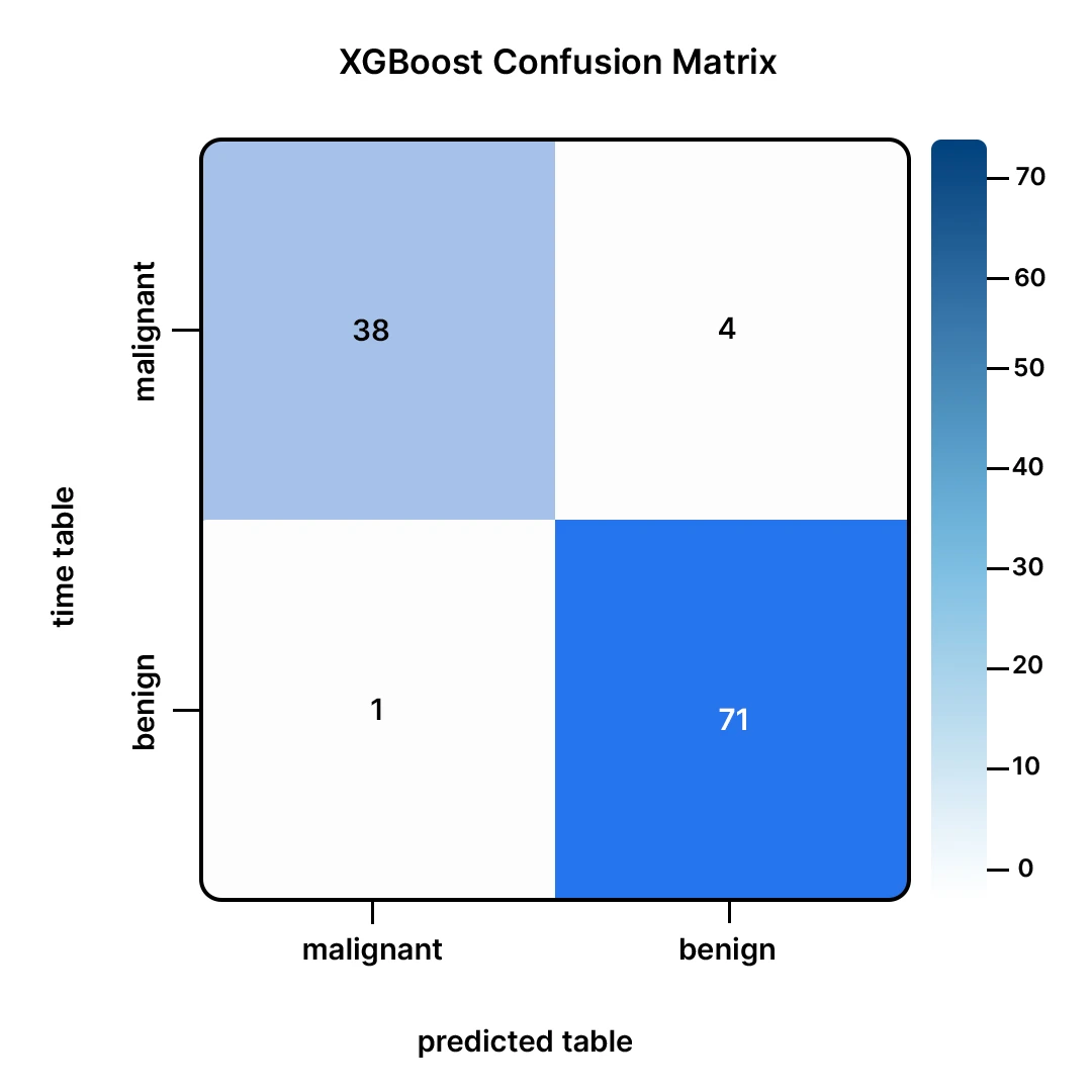
This matrix tells us:
- Out of the 43 malignant tumors (malignant), our mannequin was proper in 40 (True Positives).
- It missed 3 malignant tumors, and that is thought-about to be probably the most harmful error as a result of it’s an error made on benign tumors (False Negatives).
- Among the many 71 benign tumors (benign), our mannequin was proper on 69 (True Negatives).
- It additionally wrongly reported 2 benign tumors as most cancers (False Positives).
All in all, it is a nice efficiency. Errors made within the mannequin are minimal.
4. Tuning for Higher Efficiency
We are able to regularly squeeze extra efficiency by adjusting the hyperparameters of the mannequin. We are able to try and establish a extra optimum maxdepth, studying charge, and estimators with the assistance of the GridSearchCV.
import warnings
from sklearn.model_selection import GridSearchCV

warnings.filterwarnings('ignore', class=UserWarning, module="xgboost")

param_grid = {
   'max_depth': [3, 6],
   'learning_rate': [0.1, 0.01],
   'n_estimators': [50, 100]
}

grid_search = GridSearchCV(
   xgb.XGBClassifier(use_label_encoder=False, eval_metric="logloss", random_state=42),
   param_grid, scoring='accuracy', cv=3, verbose=1
)

grid_search.match(X_train, y_train);

print(f"Finest parameters: {grid_search.best_params_}")
best_model = grid_search.best_estimator_

# Consider the tuned mannequin
y_pred_best = best_model.predict(X_test)
best_accuracy = accuracy_score(y_test, y_pred_best)
print(f"Take a look at Accuracy with finest params: {best_accuracy*100:.2f}%")
Output:
Tuning enabled us to discover a easier (max depth of three somewhat than the default depth of 6) mannequin that achieves barely higher efficiency. This is a wonderful end result; we obtain extra accuracy with a much less advanced mannequin, and that’s much less liable to overfitting.
XGBoost consists of built-in regularization to cut back overfitting. The 2 key regularization parameters are:
- lambda (L2 regularization): reg_lambda within the scikit-learn wrapper
- alpha (L1 regularization): reg_alpha within the scikit-learn wrapper
These are official XGBoost parameters used to manage mannequin complexity.
Instance:
mannequin = xgb.XGBClassifier(
max_depth=3,
n_estimators=500,
learning_rate=0.05,
reg_lambda=2.0, # stronger L2 regularization
reg_alpha=0.5, # add L1 regularization
random_state=42,
eval_metric="logloss"
) - Improve reg_lambda when the mannequin is overfitting barely
- Improve reg_alpha if you’d like extra aggressive sparsity within the discovered weights and stronger management
Overfitting management
Think about the XGBoost coaching as carving. The scale of your instruments will depend on the depth of the timber. Deep timber are sharp instruments; they might minimize a fantastic element, however they might minimize errors within the sculpture. The amount of timber determines the period of sculpting. Extra refinements additionally imply extra timber, and as time goes on, you’re truly refining noise somewhat than refining the form. The speed of studying determines the depth of every stroke. A smaller studying charge is light sculpting: it’s slower, safer, and customarily cleaner, however requires extra strokes (extra timber).
The sculpting is the best methodology of stopping overfitting, which is to sculpt regularly and give up on the acceptable second. Virtually, that’s through the use of a decrease studying charge, extra timber, coaching by early stopping utilizing a validation set, extra sampling (2), and stronger regularisation. Select extra regularisation and sampling to make sure your mannequin isn’t overconfident within the minute particulars unlikely to look in new knowledge.
5. Understanding Function Significance
Probably the greatest issues about tree-based fashions is that they will produce studies of probably the most helpful options that had been used when it got here to creating a prediction.
# Get and plot characteristic importances
importances = best_model.feature_importances_
feature_names = knowledge.feature_names
top_indices = np.argsort(importances)[-10:][::-1]

plt.determine(figsize=(8, 6))
plt.barh(feature_names[top_indices], importances[top_indices], shade="skyblue")
plt.gca().invert_yaxis()
plt.xlabel("Significance Rating")
plt.title("Prime 10 Function Importances (XGBoost)")
plt.present()
Output:
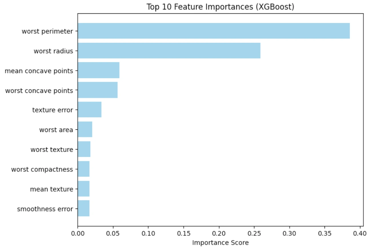
It’s clear within the plot that, among the many options related with the geometry of the tumor, the worst concave factors and the worst space are probably the most important predictors. That is in line with the medical information and makes us imagine that the mannequin is buying pertinent patterns.
When NOT to make use of XGBoost
The XGBoost is a robust device, however not essentially the suitable one. The next are examples of cases below which you’re purported to think about one thing aside from this:
- When interpretability is a strict requirement: In a regulatory or a medical context, the place you could clarify every prediction in a easy method, then a logistic regression or a bit choice tree can match higher.
- When your downside is usually linear: In case the linear mannequin already does a very good job, XGBoost may not make any important distinction with out making an attempt to be overly advanced.
- When your knowledge is unstructured (photos, uncooked audio, uncooked textual content): Deep studying architectures are likely to work with uncooked, unstructured inputs. XGBoost is optimistic within the presence of engineered (structured) options.
- When latency/reminiscence is extraordinarily constrained: An outsized, amplified mannequin could also be extra heavy than the easier fashions.
- When your dataset is extraordinarily small: XGBoost can overfit shortly on tiny datasets until you tune fastidiously.
Conclusion
We have now discovered the the reason why XGBoost is the algorithm of alternative for a lot of knowledge scientists. It’s a quick and extremely performant gradient boosting implementation. We mentioned the reasoning behind its sequential and error-correcting course of and in contrast it to different fashions which can be widespread.
In our sensible instance, XGBoost was in a position to carry out fairly properly even with minimal tuning. The complexity of XGBoost could also be very obscure, however it turns into comparatively simple to adapt to XGBoost utilizing up to date libraries. It’s potential to make it greater than a part of your machine studying arsenal, as with follow, it will likely be ready to deal with your most difficult knowledge issues.
Ceaselessly Requested Questions
A. Not all the time. When toyed with, XGBoost tends to work higher however with default parameters. Random Forest is extra resilient, much less delicate to overfitting and tends to work fairly properly.
A. No. Much like different fashions that depend on choice timber, XGBoost doesn’t care concerning the measurement of your options, thus you don’t want to scale or normalize your options.
A. It’s an acronym of eXtreme Gradient Boosting and it implies that the library is aimed toward maximizing the computational velocity and fashions efficiency.
A. Staple items are typically sophisticated. Although, with the scikit-learn API, implementation could be very easy to any Python person.
A. Sure, completely. XGBoost is extremely versatile and comprises highly effective regression (predicting steady values) and rating duties implementations.
Harsh Mishra is an AI/ML Engineer who spends extra time speaking to Giant Language Fashions than precise people. Keen about GenAI, NLP, and making machines smarter (in order that they don’t substitute him simply but). When not optimizing fashions, he’s in all probability optimizing his espresso consumption. 🚀☕
Login to proceed studying and luxuriate in expert-curated content material.
