A Information to Zero-Day Assault Detection with Denoising Autoencoders

Zero-day assaults are among the many most critical cybersecurity threats. They exploit beforehand unknown vulnerabilities, permitting them to bypass present intrusion detection programs (IDS). Conventional signature-based IDS fails right here because it relies on the recognized assault sample.  To detect such a sort of assault, fashions must be taught what regular community behaviour appears like and flag robotically when it deviates from it.

A promising resolution is the applying of the Denoising Autoencoder (DAE), which is an unsupervised deep studying mannequin designed to be taught strong representations of regular visitors. The primary concept is that by barely corrupting the enter throughout coaching, DAE learns to reconstruct the unique, clear model of information.  This forces the mannequin to seize the important illustration of the info fairly than memorizing noise. When confronted with an unseen zero-day assault, the loss perform, i.e., reconstruction error spikes, makes the anomaly detection. On this article, we are going to see how one can use a DAE on the UNSW-NB15 dataset for zero-day assault detection.

Denoising Autoencoders: The Core Thought

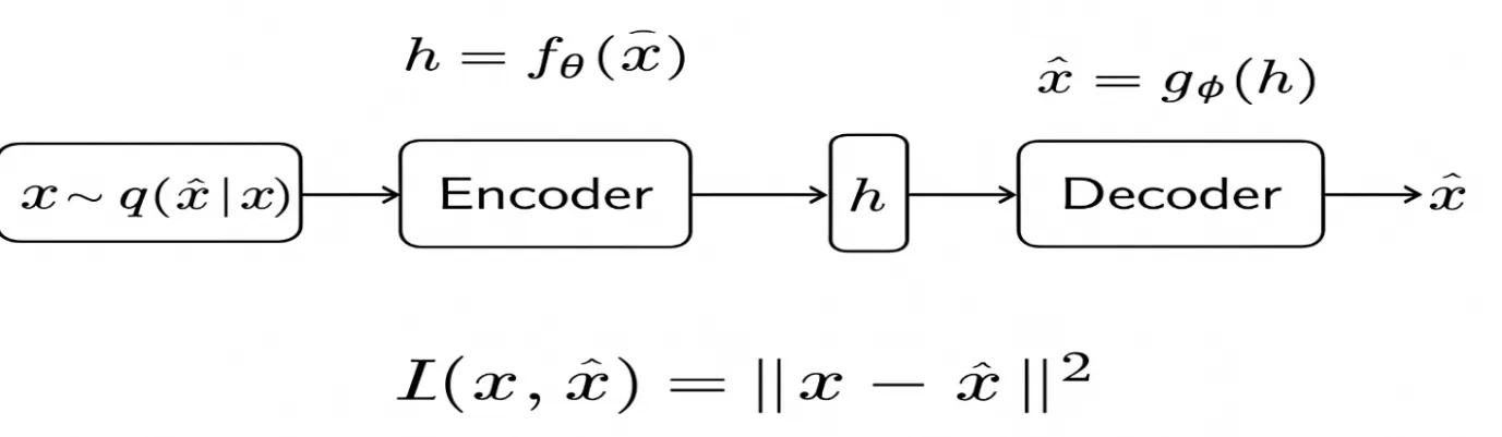
In denoising autoencoders, we deliberately add noise to the enter earlier than passing it to the encoder. The community then learns to reconstruct the unique, clear enter. To encourage the mannequin to give attention to significant options fairly than particulars, we corrupt the enter information utilizing random noise. We specific this mathematically as:

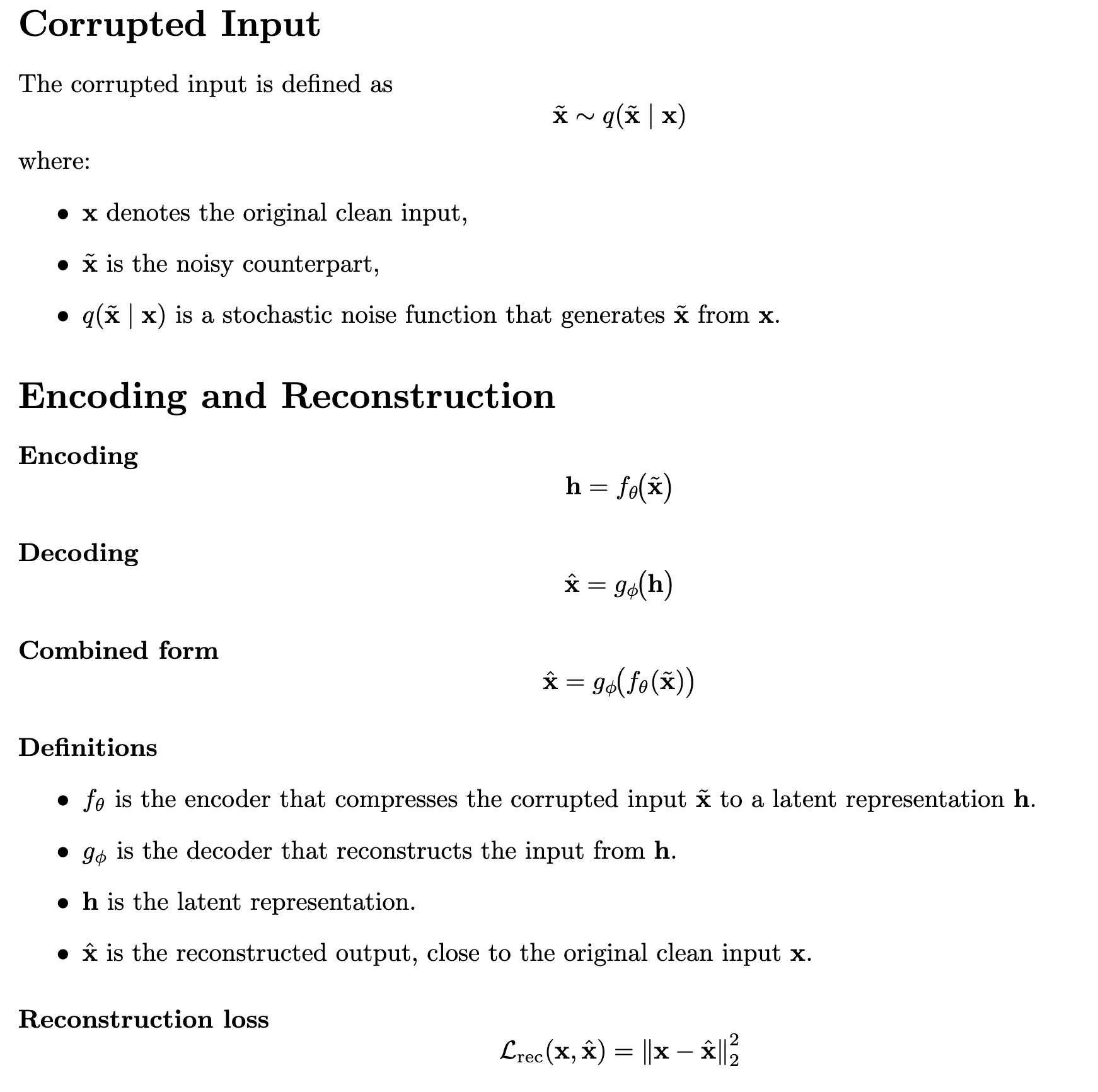
The reconstruction loss is often known as the loss perform, which evaluates the distinction between the unique enter information x and the reconstructed output information x̂.  The decrease reconstruction error signifies that the mannequin ignores noise and retains important options of the enter. The beneath diagrammatic illustration reveals the diagrammatic illustration of the Denoising Autoencoders.

Instance: Binary Enter Case

Take into account binary inputs (x ∈ {0,1}. With chance q, we flip a bit or set it to 0; in any other case, we depart it unchanged. If we allowed the mannequin to reduce the error with respect to the corrupted enter x, it might merely be taught to repeat the corruption. However as a result of we drive it to reconstruct the true x, it should infer the lacking data from the relationships between options. This results in a DAE mannequin strong they generalizes past memorization and be taught a deeper construction in regards to the enter. to noise and improves generalization throughout testing. Within the context of cybersecurity, a denoising Autoencoder affords the flexibility to detect unseen or zero-day assaults that deviate from the conventional patterns.

Case Research: Zero-Day Assault Detection with Denoising Autoencoders

This instance illustrates how a Denoising Autoencoder can detect zero-day assaults within the UNSW-NB15 dataset. We practice the mannequin to be taught the underlying construction of regular visitors with out letting the anomalous information affect it. Throughout inference, the mannequin evaluates the community flows that considerably deviate from regular patterns, corresponding to these related to zero-day assaults, leading to excessive reconstruction error, enabling anomaly detection.

Step 1. Dataset Overview

The UNSW-NB15 dataset is a benchmark dataset that’s used to judge the efficiency of the Intrusion Detection System. It consists of regular samples and 9 assault lessons, together with Fuzzers, Shellcode, and Exploits. For simulating zero-day assaults, we practice solely on regular visitors and maintain out the Shellcode assault for testing. This ensures that the mannequin is evaluated on beforehand unseen assault behaviour.

Step 2. Import Libraries & Load Dataset

We import the required libraries and cargo the UNSW-NB15 dataset. We then carry out numeric preprocessing, separate the labels and categorical options, and focus solely on regular visitors for coaching.

import pandas as pd

import numpy as np

import matplotlib.pyplot as plt

from sklearn.model_selection import train_test_split

from sklearn.preprocessing import StandardScaler, OneHotEncoder

from sklearn.compose import ColumnTransformer

from sklearn.metrics import roc_curve, auc

import tensorflow as tf

from tensorflow. keras import layers, Mannequin

from tensorflow. keras.callbacks import EarlyStopping

# Load UNSW-NB15 dataset

df = pd. read_csv("UNSW_NB15.csv")

print ("Dataset form:", df. form)

print (df [['label’, ‘attack cat']].head())

 Output: 

Dataset form: (254004, 43)
First 5 rows of ['label','attack_cat']:
     label     attack_cat
0      0          Regular
1      0          Regular
2      0          Regular
3      0          Regular
4      1         Shellcode

The output reveals the dataset has 254,004 rows and 43 columns. The label 0 for regular flows and 1 for assault flows. The fifth row is a Shellcode assault, which we’re utilizing for the detection of the as our zero-day assault.

Step 3. Preprocess Information

# Outline goal

y = df['label']

X = df.drop(columns=['label'])

# Regular visitors for coaching

normal_data = X[y == 0]

# Zero-day visitors (Shellcode) for testing

zero_day_data = df[df['attack_cat'] == 'Shellcode'].drop(columns=['label','attack_cat'])

# Determine numeric and categorical options

numeric_features = normal_data.select_dtypes(embody=['int64','float64']).columns

categorical_features = normal_data.select_dtypes(embody=['object']).columns

# Preprocessing pipeline: scale numerics, one-hot encode categoricals

preprocessor = ColumnTransformer([

    ("num", StandardScaler(), numeric_features),

    ("cat", OneHotEncoder(handle_unknown="ignore", sparse=False), categorical_features)

])

# Match solely on regular visitors

X_normal = preprocessor.fit_transform(normal_data)

# Prepare-validation break up

X_train, X_val = train_test_split(X_normal, test_size=0.2, random_state=42)

print("Coaching information form:", X_train.form)

print("Validation information form:", X_val.form)

Output:

Coaching information form:    (160000, 71)
Validation information form:  ( 40000, 71)

The label is dropped and solely benign samples, i.e. i == 0 are chosen. There are 37 numeric options – one-hot encoded 4 categorical options, which grow to be the 71 complete enter dimensions.

Step 4. Outline Optimized Denoising Autoencoder

We add Gaussian Noise to inputs to drive the community to be taught strong options. Batch Normalization stabilizes coaching, and a small bottleneck layer (16 items) encourages compact latent representations.

input_dim = X_train. form [1]

inp = layers.Enter(form=(input_dim,))

noisy = layers. GaussianNoise(0.1)(inp)  # Corrupt enter barely

# Encoder

x = layers.Dense(64, activation='relu')(noisy)

x = layers. BatchNormalization()(x)  # Stabilize coaching

bottleneck = layers.Dense(16, activation='relu')(x)

# Decoder

x = layers.Dense(64, activation='relu')(bottleneck)

x = layers. BatchNormalization()(x)

out = layers.Dense(input_dim, activation='linear')(x)  # Use linear for standardized enter

autoencoder = Mannequin(inputs=inp, outputs=out)

autoencoder. compile(optimizer="adam", loss="mse")

autoencoder.abstract()

Output:

Mannequin: "mannequin"
_________________________________________________________________
Layer (kind)                        Output Form                          Param #
=================================================================
input_1 (InputLayer)                [(None, 71)]                             0
gaussian_noise (GaussianNoise)      (None, 71)                        0
dense (Dense)                       (None, 64)                                4,608
batch_normalization (BatchNormalization) (None, 64)        128
dense_1 (Dense)                     (None, 16)                              1,040
dense_2 (Dense)                     (None, 64)                               1,088
batch_normalization_1 (BatchNormalization) (None, 64)     128
dense_3 (Dense)                     (None, 71)                               4,615
=================================================================
Complete params: 11,607  
Trainable params: 11,351  
Non-trainable params:   256  
_________________________________________________________________

Step 5. Prepare the Mannequin with Early Stopping

# Early stopping to keep away from overfitting

es = EarlyStopping(monitor="val_loss", endurance=3, restore_best_weights=True)

print("Coaching began...")

historical past = autoencoder.match (

    X_train, X_train,

    epochs=50,

    batch_size=512,  # bigger batch for sooner coaching

    validation_data=(X_val, X_val),

    shuffle=True,

    callbacks=[es]

)

print ("Coaching accomplished!")

Coaching Loss Curve

plt.plot(historical past.historical past['loss'], label="Prepare Loss")

plt.plot(historical past.historical past['val_loss'], label="Val Loss")

plt.xlabel("Epochs")

plt.ylabel("MSE Loss")

plt.legend()

plt.title("Coaching vs Validation Loss")

plt.present()

Output:

Coaching began...
Epoch 1/50
313/313 [==============================] - 2s  6ms/step - loss: 0.0254 - val_loss: 0.0181
Epoch 2/50
313/313 [==============================] - 2s  6ms/step - loss: 0.0158 - val_loss: 0.0145
Epoch 3/50
313/313 [==============================] - 2s  6ms/step - loss: 0.0123 - val_loss: 0.0127
Epoch 4/50
313/313 [==============================] - 2s  6ms/step - loss: 0.0106 - val_loss: 0.0108
Epoch 5/50
313/313 [==============================] - 2s  6ms/step - loss: 0.0094 - val_loss: 0.0097
Epoch 6/50
313/313 [==============================] - 2s  6ms/step - loss: 0.0086 - val_loss: 0.0085
Epoch 7/50
313/313 [==============================] - 2s  6ms/step - loss: 0.0082 - val_loss: 0.0083
Epoch 8/50
313/313 [==============================] - 2s  6ms/step - loss: 0.0080 - val_loss: 0.0086
Restoring mannequin weights from the tip of one of the best epoch: 7.
Epoch 00008: early stopping
Coaching accomplished!

Step 6. Zero-Day Detection

# Rework datasets

X_normal_test = preprocessor.rework(normal_data)

X_zero_day_test = preprocessor.rework(zero_day_data)

# Compute reconstruction errors

recon_normal = np.imply(np.sq.(X_normal_test - autoencoder.predict(X_normal_test, batch_size=512)), axis=1)

recon_zero = np.imply(np.sq.(X_zero_day_test - autoencoder.predict(X_zero_day_test, batch_size=512)), axis=1)

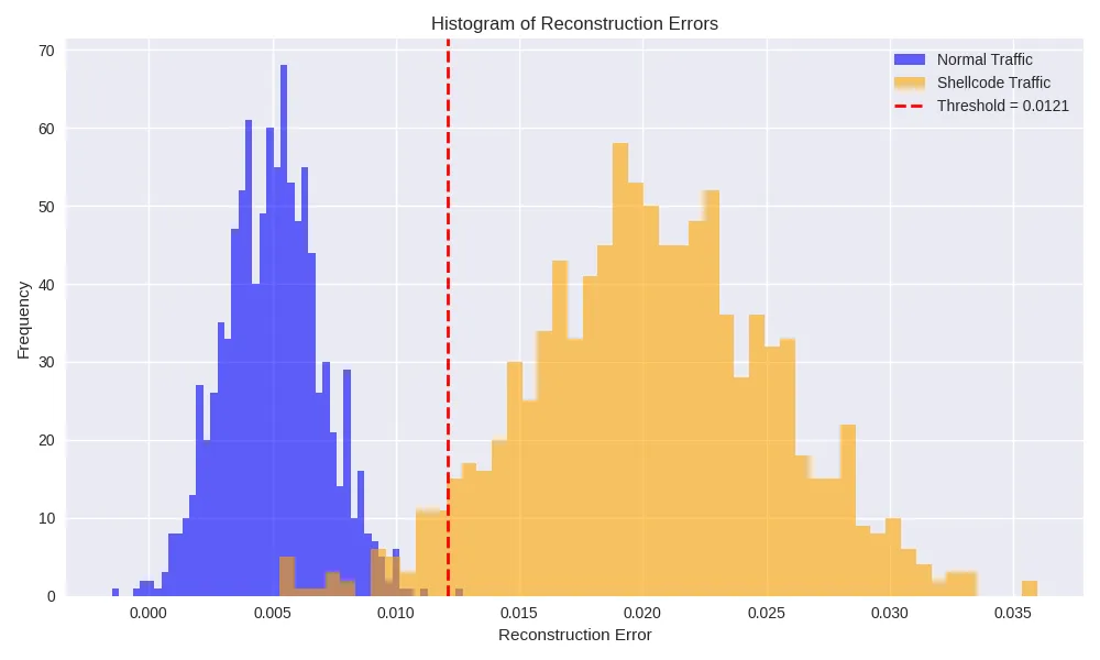
# Threshold: ninety fifth percentile of regular errors

threshold = np.percentile(recon_normal, 95)

print("Threshold:", threshold)

print("False Alarm Price (Regular flagged as anomaly):", np.imply(recon_normal > threshold))

print("Detection Price (Zero-Day detected):", np.imply(recon_zero > threshold))

Output:

Threshold: 0.0121
False Alarm Price (regular→anomaly): 0.0480
Detection Price (Shellcode zero-day): 0.9150

We set the edge on the ninety fifth percentile of benign-flow errors. 4.8% of regular visitors is flagged as false positives, whereas roughly 91.5% of Shellcode flows exceed the edge and are appropriately recognized as true positives.

Step 7. Visualization

Histogram of Reconstruction Errors

plt. determine(figsize=(8,5))

plt.hist(recon_normal, bins=50, alpha=0.6, label="Regular")

plt.hist(recon_zero, bins=50, alpha=0.6, label="Zero-Day (Shellcode)")

plt.axvline(threshold, shade="crimson", linestyle="--", label="Threshold")

plt.xlabel("Reconstruction Error")

plt.ylabel("Frequency")

plt.legend()

plt.title("Regular vs Zero-Day Error Distribution")

plt.present()

Output:

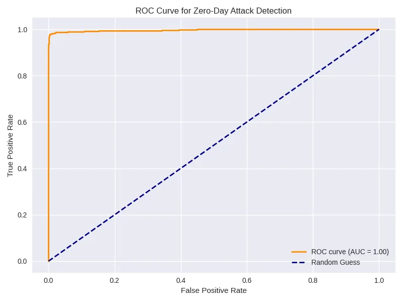
ROC Curve

y_true = np.concatenate([np.zeros_like(recon_normal), np.ones_like(recon_zero)])

y_scores = np.concatenate([recon_normal, recon_zero])

fpr, tpr, _ = roc_curve(y_true, y_scores)

roc_auc = auc(fpr, tpr)

plt.plot(fpr, tpr, label=f"AUC = {roc_auc:.2f}")

plt.plot([0,1],[0,1],'--')

plt.xlabel("False Optimistic Price")

plt.ylabel("True Optimistic Price")

plt.legend()

plt.title("ROC Curve for Zero-Day Detection")

plt.present()

Output:

Limitations

Listed here are the constraints of this:

• DAEs detect anomalies however don’t classify assault sorts.
• Choosing an acceptable threshold relies on the collection of the dataset and should contain fine-tuning.
• Works finest when skilled solely on regular visitors.

Key Takeaways

• Denoising Autoencoders are efficient in detecting unseen zero-day assaults.
• Coaching stability improves with BatchNormalization, bigger batch sizes, and early stopping.
• Visualizations (loss curves, error histograms, ROC) make mannequin behaviour interpretable. 
• This method might be carried out in a hybrid manner for assault classification or a real-time community intrusion detection system.

Conclusion

This tutorial demonstrates how a Denoising Autoencoder can detect zero-day assaults in community visitors utilizing the UNSW-NB15 dataset. By studying a sturdy sample of regular visitors, the mannequin flags anomalies in unseen assault information. DAE alone supplies a powerful basis for contemporary Intrusion Detection Programs, and might be mixed with superior architectures or supervised classifiers to construct a complete intrusion detection system.

Learn extra: AI in Cybersecurity

Ceaselessly Requested Questions

Assistant Professor | Info Expertise | PhD Scholar

I’m an Assistant Professor within the Info Expertise division at NMIET, Talegaon, Pune, with over 16 years of expertise. I maintain a B.E. from Sant Gadge Baba College, Amravati, an M.E. from Savitribai Phule Pune College, and am at the moment pursuing a PhD in Pc Engineering from Mumbai College.

I focus on Synthetic Intelligence and Pure Language Processing, supported by certifications in Immediate Engineering for Generative AI, AI Productiveness Hacks, and Generative AI for Artistic Content material from LinkedIn.
Keen about bridging trade and academia, I give attention to equipping college students with sensible expertise to excel within the evolving expertise panorama.