SQL and Python for Retail

Think about it’s Black Friday morning, and your flagship retailer is offered out of the most popular merchandise of the season by 10 AM, whereas your warehouse is full of gadgets that no one needs. Sound acquainted? In right now’s retail market, producing correct demand forecasts will not be solely fascinating; it’s what separates revenue from loss. Easy shifting averages or “intestine really feel” strategies received’t work within the advanced trendy retail offers with seasonality, promotional actions, climate impacts, and quickly shifting client preferences.

On this complete information, we are going to information you thru the method of constructing a requirement forecasting system that is able to be put into manufacturing and is ready to forecast demand on thousands and thousands of SKUs throughout a whole bunch of places, enabling you to supply what your small business wants greater than something: accuracy.

Why Does This Matter?

With trendy retailers, the challenges they fight are distinctive constructions:

• Scale: Hundreds of merchandise × A whole lot of places = Tens of millions of forecasts daily
• Complexity: Climate, holidays, promotions, and developments all impression demand, however in several methods
• Velocity: Stock choices can not watch for handbook evaluation
• Price: Poor forecasts straight have an effect on the underside line via extra stock or stockouts

Let’s create a system to resist these challenges.

Half 1: Constructing the Knowledge Basis

Earlier than we dive into advanced algorithms, let’s construct a strong information basis, as demand forecasts begin with an excellent information construction.

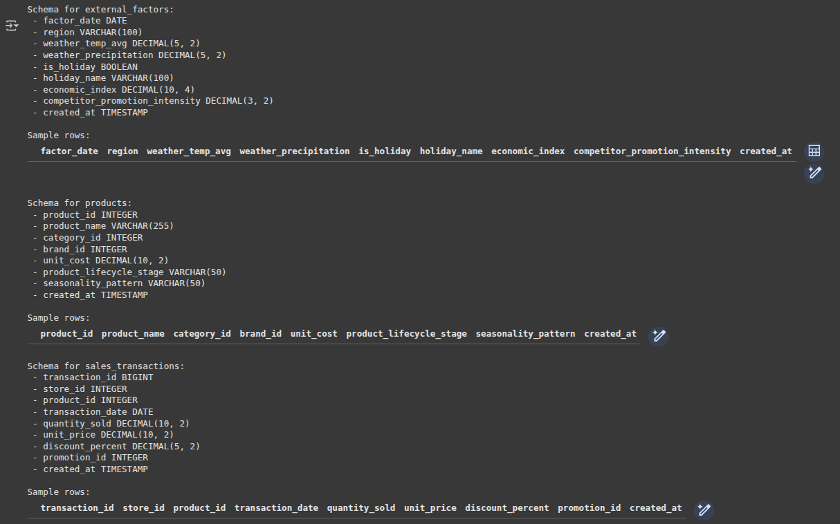
Database Schema Design

First, let’s create tables that seize all the knowledge we’d like for forecasting:

1. Core gross sales transaction desk

CREATE TABLE sales_transactions (

    transaction_id BIGINT PRIMARY KEY,

    store_id INT NOT NULL,

    product_id INT NOT NULL,

    transaction_date DATE NOT NULL,

    quantity_sold DECIMAL(10,2) NOT NULL,

    unit_price DECIMAL(10,2) NOT NULL,

    discount_percent DECIMAL(5,2) DEFAULT 0,

    promotion_id INT,

    created_at TIMESTAMP DEFAULT CURRENT_TIMESTAMP

);

2. Product grasp information

CREATE TABLE merchandise (

    product_id INT PRIMARY KEY,

    product_name VARCHAR(255) NOT NULL,

    category_id INT NOT NULL,

    brand_id INT,

    unit_cost DECIMAL(10,2),

    product_lifecycle_stage VARCHAR(50), -- 'new', 'progress', 'mature', 'decline'

    seasonality_pattern VARCHAR(50), -- 'spring', 'summer time', 'fall', 'winter', 'none'

    created_at TIMESTAMP DEFAULT CURRENT_TIMESTAMP

);

Why this construction?
It’s not solely capturing gross sales information, but additionally considering context associated to the demand: product life-cycle, seasonality patterns, and pricing data. The context is of nice significance when offering an correct forecast. 

Exterior Components Desk

Demand doesn’t exist in a vacuum. Exterior components usually drive important demand change:

1. Exterior components that affect demand

CREATE TABLE external_factors (

    factor_date DATE PRIMARY KEY,

    area VARCHAR(100),

    weather_temp_avg DECIMAL(5,2),

    weather_precipitation DECIMAL(5,2),

    is_holiday BOOLEAN DEFAULT FALSE,

    holiday_name VARCHAR(100),

    economic_index DECIMAL(10,4),

    competitor_promotion_intensity DECIMAL(3,2), -- 0-1 scale

    created_at TIMESTAMP DEFAULT CURRENT_TIMESTAMP

);

Output:

Professional tip: Begin gathering exterior information even in case you’re not utilizing it but. Climate information for final yr is inconceivable to get, but it surely could possibly be essential for forecasting seasonal merchandise.

Half 2: Superior Characteristic Engineering in SQL

That is the important thing level on this course of. Right here we are going to take some gross sales information and create options that machine-learning algorithms can use to establish patterns.

Temporal-Based mostly Options: The Basis

Temporal patterns are the spine of demand prediction. Let’s extract some significant time options:

1. Extract complete time-based options

WITH time_features AS (

    SELECT 

        store_id,

        product_id,

        transaction_date,

        SUM(quantity_sold) as total_quantity,

        -- Fundamental time parts

        EXTRACT(YEAR FROM transaction_date) as yr,

        EXTRACT(MONTH FROM transaction_date) as month,

        EXTRACT(DOW FROM transaction_date) as day_of_week, -- 0=Sunday

        EXTRACT(WEEK FROM transaction_date) as week_of_year,

        -- Weekend indicator

        CASE 

            WHEN EXTRACT(DOW FROM transaction_date) IN (0, 6) THEN 1 

            ELSE 0 

        END as is_weekend,

        -- Cyclical encoding for seasonality (key perception!)

        SIN(2 * PI() * EXTRACT(DOY FROM transaction_date) / 365.25) as day_of_year_sin,

        COS(2 * PI() * EXTRACT(DOY FROM transaction_date) / 365.25) as day_of_year_cos

    FROM sales_transactions 

    GROUP BY store_id, product_id, transaction_date

)

SELECT * FROM time_features;

Output:

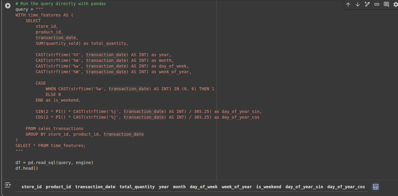
Why use cyclical encoding?
Typical approaches contemplate December 31 and January 1 fully unrelated (365 vs 1). Cyclical encoding with sine/cosine reveals that, though numerically totally different, these values are adjoining within the seasonal cycle.

Lag Options: Studying from the Previous

Typically, historic efficiency is predictive of future efficiency. This leads us to creating options that look again at historical past:

1. Create lag and rolling window options

WITH lag_features AS (

    SELECT 

        *,

        -- Earlier day, week, month, and yr values

        LAG(total_quantity, 1) OVER (

            PARTITION BY store_id, product_id 

            ORDER BY transaction_date

        ) as quantity_lag_1d,

        LAG(total_quantity, 7) OVER (

            PARTITION BY store_id, product_id 

            ORDER BY transaction_date

        ) as quantity_lag_7d,

        LAG(total_quantity, 365) OVER (

            PARTITION BY store_id, product_id 

            ORDER BY transaction_date

        ) as quantity_lag_365d,

        -- 7-day shifting common

        AVG(total_quantity) OVER (

            PARTITION BY store_id, product_id 

            ORDER BY transaction_date 

            ROWS BETWEEN 6 PRECEDING AND CURRENT ROW

        ) as quantity_ma_7d

    FROM time_features

)

SELECT * FROM lag_features;

Enterprise perception: The total-year delay captures year-over-year comparables routinely. For those who offered 100 winter coats on the identical day final yr, that gives useful context for this yr’s forecast.

Seasonal and Development Evaluation

Let’s establish underlying patterns within the information by way of a question:

1. Superior seasonal and development options

WITH seasonal_features AS (

    SELECT 

        *,

        -- 12 months-over-year progress fee

        CASE 

            WHEN quantity_lag_365d > 0 THEN 

                (total_quantity - quantity_lag_365d) / quantity_lag_365d

            ELSE NULL

        END as yoy_growth_rate,

        -- Seasonal power (how does right now examine to historic common for this month?)

        total_quantity / NULLIF(

            AVG(total_quantity) OVER (

                PARTITION BY store_id, product_id, month

            ), 0

        ) as seasonal_index_monthly,

        -- Volatility measure

        STDDEV(total_quantity) OVER (

            PARTITION BY store_id, product_id 

            ORDER BY transaction_date 

            ROWS BETWEEN 29 PRECEDING AND CURRENT ROW

        ) / NULLIF(quantity_ma_7d, 0) as coefficient_of_variation

    FROM lag_features

)

SELECT * FROM seasonal_features;

Key perception: The seasonal index tells us if right now’s gross sales are above or beneath a traditional sample for the time of yr.  A worth of 1.5 means gross sales are 50% above the seasonal common.

Half 3: Python Machine Studying Pipeline

Now, let’s construct a machine studying pipeline that may assist us flip these options into correct forecasts.

Core Forecasting Class

Right here’s the essential foundational class of our demand forecasts system:

import pandas as pd

import numpy as np

from datetime import datetime, timedelta

from sklearn.ensemble import RandomForestRegressor

from sklearn.model_selection import TimeSeriesSplit

import xgboost as xgb

import warnings

warnings.filterwarnings('ignore')

class RetailDemandForecaster:

    def __init__(self, connection_string):

        self.connection_string = connection_string

        self.fashions = {}

        self.feature_columns = []

        self.skilled = False

    def load_and_prepare_data(self, start_date, end_date):

        """Load information with all our engineered options"""

        # In observe, this might execute our SQL characteristic engineering

        # For now, let's simulate ready information

        print(f"Loading information from {start_date} to {end_date}")

        # This might include the results of our SQL queries above

        # with all of the time-based, lag, and seasonal options

        return self._simulate_prepared_data()

    def _simulate_prepared_data(self):

        """Simulate ready information for demo functions"""

        dates = pd.date_range('2022-01-01', '2024-01-01', freq='D')

        np.random.seed(42)

        information = []

        for store_id in [1, 2, 3]:

            for product_id in [101, 102, 103]:

                for date in dates:

                    # Simulate seasonal sample

                    seasonal_factor = 1 + 0.3 * np.sin(2 * np.pi * date.dayofyear / 365)

                    base_demand = 50 + np.random.regular(0, 10)

                    information.append({

                        'store_id': store_id,

                        'product_id': product_id,

                        'date': date,

                        'total_quantity': max(0, base_demand * seasonal_factor),

                        'day_of_week': date.dayofweek,

                        'month': date.month,

                        'is_weekend': 1 if date.dayofweek >= 5 else 0,

                        'day_of_year_sin': np.sin(2 * np.pi * date.dayofyear / 365),

                        'day_of_year_cos': np.cos(2 * np.pi * date.dayofyear / 365)

                    })

        return pd.DataFrame(information)

What’s the reasoning behind this association?
We’re establishing a category that’s simple to increase and straightforward to keep up. The separation of knowledge loading from mannequin coaching makes it simpler to discover totally different approaches.

Characteristic Engineering Pipeline

Let’s add some superior characteristic engineering capabilities:

def create_advanced_features(self, df):

    """Create superior options which are arduous to do in SQL"""

    df_copy = df.copy().sort_values(['store_id', 'product_id', 'date'])

    # Create lag options effectively

    for store_prod, group in df_copy.groupby(['store_id', 'product_id']):

        masks = (df_copy['store_id'] == store_prod[0]) & (df_copy['product_id'] == store_prod[1])

        # A number of lag intervals

        for lag_days in [1, 7, 14, 30]:

            df_copy.loc[mask, f'quantity_lag_{lag_days}d'] = group['total_quantity'].shift(lag_days)

        # Rolling statistics

        df_copy.loc[mask, 'quantity_rolling_mean_7d'] = group['total_quantity'].rolling(7, min_periods=1).imply()

        df_copy.loc[mask, 'quantity_rolling_std_7d'] = group['total_quantity'].rolling(7, min_periods=1).std()

        # Development options (velocity and acceleration)

        df_copy.loc[mask, 'quantity_velocity'] = group['total_quantity'].diff()

        df_copy.loc[mask, 'quantity_acceleration'] = group['total_quantity'].diff().diff()

    # Fill NaN values

    numeric_columns = df_copy.select_dtypes(embrace=[np.number]).columns

    df_copy[numeric_columns] = df_copy[numeric_columns].fillna(methodology='ffill').fillna(0)

    return df_copy

# Add this methodology to the RetailDemandForecaster class

RetailDemandForecaster.create_advanced_features = create_advanced_features

Useful Tip: We’re calculating options by the store-product pairing in order that we don’t leak data between merchandise or places. 

Coaching the Mannequin with an Ensemble Method

At this level in our challenge, we are going to now prepare numerous fashions and fuse them to achieve superior accuracy:

def train_models(self, df, target_column='total_quantity', forecast_horizons=[1, 7, 14]):

    """Practice ensemble of fashions for a number of forecast horizons"""

    # Put together options and targets

    feature_cols = [col for col in df.columns 

                   if col not in ['date', 'store_id', 'product_id', target_column]]

    X = df[feature_cols]

    self.feature_columns = feature_cols

    # Practice separate fashions for every forecast horizon

    for horizon in forecast_horizons:

        print(f"Coaching fashions for {horizon}-day forecast...")

        # Create goal variable (future values)

        y = df.groupby(['store_id', 'product_id'])[target_column].shift(-horizon)

        # Take away rows the place goal is NaN

        valid_rows = ~y.isna()

        X_clean = X[valid_rows]

        y_clean = y[valid_rows]

        if len(X_clean) == 0:

            proceed

        # Initialize fashions

        fashions = {

            'random_forest': RandomForestRegressor(n_estimators=100, random_state=42, n_jobs=-1),

            'xgboost': xgb.XGBRegressor(n_estimators=100, random_state=42, n_jobs=-1)

        }

        self.fashions[f'horizon_{horizon}'] = {}

        # Practice every mannequin with time collection cross-validation

        tscv = TimeSeriesSplit(n_splits=5)

        for model_name, mannequin in fashions.gadgets():

            print(f"  Coaching {model_name}...")

            # Cross-validation scores

            cv_scores = []

            for train_idx, val_idx in tscv.cut up(X_clean):

                X_train, X_val = X_clean.iloc[train_idx], X_clean.iloc[val_idx]

                y_train, y_val = y_clean.iloc[train_idx], y_clean.iloc[val_idx]

                mannequin.match(X_train, y_train)

                y_pred = mannequin.predict(X_val)

                # Calculate MAPE (Imply Absolute Share Error)

                mape = np.imply(np.abs((y_val - y_pred) / y_val)) * 100

                cv_scores.append(mape)

            avg_mape = np.imply(cv_scores)

            print(f"    Cross-validation MAPE: {avg_mape:.2f}%")

            # Practice remaining mannequin on all information

            mannequin.match(X_clean, y_clean)

            self.fashions[f'horizon_{horizon}'][model_name] = mannequin

    self.skilled = True

    print("Mannequin coaching accomplished!")

# Add this methodology to the RetailDemandForecaster class

RetailDemandForecaster.train_models = train_models

Why ensemble fashions?
Totally different algorithms seize totally different patterns. Random Forest does a superb job of dealing with nonlinear relationships, and XGBoost captures delicate interactions between options very effectively.

Making the Predictions:

Now we are going to add the power to foretell:

def predict(self, df, forecast_horizons=[1, 7, 14]):

    """Generate forecasts for a number of horizons"""

    if not self.skilled:

        elevate ValueError("Fashions have to be skilled earlier than making predictions")

    X = df[self.feature_columns]

    predictions = {}

    for horizon in forecast_horizons:

        horizon_key = f'horizon_{horizon}'

        if horizon_key not in self.fashions:

            proceed

        horizon_predictions = []

        # Get predictions from every mannequin

        for model_name, mannequin in self.fashions[horizon_key].gadgets():

            pred = mannequin.predict(X)

            horizon_predictions.append(pred)

        # Ensemble: easy common (might be made extra subtle)

        ensemble_pred = np.imply(horizon_predictions, axis=0)

        predictions[f'forecast_{horizon}d'] = np.most(0, ensemble_pred)  # Guarantee non-negative

    return pd.DataFrame(predictions, index=df.index)

# Add this methodology to the RetailDemandForecaster class

RetailDemandForecaster.predict = predict

Half 4: Mannequin Analysis and Insights

Let’s implement business-relevant analysis metrics:

def evaluate_performance(self, precise, predicted):

    """Calculate complete efficiency metrics"""

    metrics = {}

    for col in predicted.columns:

        if col in precise.columns:

            y_true = precise[col].values

            y_pred = predicted[col].values

            # Take away any NaN values

            valid_mask = ~(np.isnan(y_true) | np.isnan(y_pred))

            y_true_clean = y_true[valid_mask]

            y_pred_clean = y_pred[valid_mask]

            if len(y_true_clean) == 0:

                proceed

            # Enterprise-relevant metrics

            mae = np.imply(np.abs(y_true_clean - y_pred_clean))

            mape = np.imply(np.abs((y_true_clean - y_pred_clean) / np.most(y_true_clean, 1))) * 100

            bias = np.imply(y_pred_clean - y_true_clean)

            # Forecast accuracy (complement of MAPE)

            accuracy = 100 - mape

            metrics[col] = {

                'MAE': mae,

                'MAPE': mape,

                'Bias': bias,

                'Accuracy': accuracy

            }

    return metrics

# Add this methodology to the RetailDemandForecaster class

RetailDemandForecaster.evaluate_performance = evaluate_performance

Why these metrics?

• MAE (Imply Absolute Error): unobtrusive to learn in enterprise language
• MAPE (Imply Absolute Share Error): We will examine merchandise
• Bias: to indicate whether or not we’re systematically over- or under-forecasting
• Accuracy: easy % that enterprise stakeholders perceive

Characteristic Significance Evaluation

Understanding what drives demand is as vital as predicting it:

def analyze_feature_importance(self, top_n=10):

    """Analyze what options are most vital for forecasting"""

    if not self.skilled:

        return {}

    importance_analysis = {}

    for horizon_key, horizon_models in self.fashions.gadgets():

        importance_analysis[horizon_key] = {}

        for model_name, mannequin in horizon_models.gadgets():

            if hasattr(mannequin, 'feature_importances_'):

                # Get characteristic significance

                importance_df = pd.DataFrame({

                    'characteristic': self.feature_columns,

                    'significance': mannequin.feature_importances_

                }).sort_values('significance', ascending=False)

                importance_analysis[horizon_key][model_name] = importance_df.head(top_n)

    return importance_analysis

# Add this methodology to the RetailDemandForecaster class

RetailDemandForecaster.analyze_feature_importance = analyze_feature_importance

Half 5: Manufacturing Deployment

Let’s construct a easy Flask API for serving predictions:

from flask import Flask, request, jsonify

import joblib

from datetime import datetime

app = Flask(__name__)

# Load skilled mannequin (in manufacturing, this might be completed at startup)

attempt:

    forecaster = joblib.load('fashions/retail_forecaster.pkl')

    print("Mannequin loaded efficiently")

besides:

    forecaster = None

    print("Warning: Couldn't load mannequin")

@app.route('/well being', strategies=['GET'])

def health_check():

    """Easy well being test endpoint"""

    standing="wholesome" if forecaster will not be None else 'unhealthy'

    return jsonify({

        'standing': standing,

        'timestamp': datetime.now().isoformat(),

        'model_loaded': forecaster will not be None

    })

@app.route('/forecast', strategies=['POST'])

def get_forecast():

    """Predominant forecasting endpoint"""

    if forecaster is None:

        return jsonify({'error': 'Mannequin not accessible'}), 503

    attempt:

        # Parse request

        information = request.json

        store_id = information.get('store_id')

        product_id = information.get('product_id')

        if not store_id or not product_id:

            return jsonify({'error': 'store_id and product_id are required'}), 400

        # In manufacturing, you'd fetch latest information and generate options

        # For demo, we'll simulate this

        recent_data = simulate_recent_data(store_id, product_id)

        # Generate forecast

        forecast = forecaster.predict(recent_data)

        return jsonify({

            'store_id': store_id,

            'product_id': product_id,

            'forecasts': forecast.iloc[0].to_dict(),

            'generated_at': datetime.now().isoformat()

        })

    besides Exception as e:

        return jsonify({'error': str(e)}), 500

def simulate_recent_data(store_id, product_id):

    """Simulate latest information for forecasting (change with actual information loading)"""

    # This might usually load the final 30-60 days of knowledge

    # and apply the identical characteristic engineering pipeline

    import pandas as pd

    import numpy as np

    # Create dummy information with required options

    information = pd.DataFrame({

        'store_id': [store_id],

        'product_id': [product_id],

        'day_of_week': [datetime.now().dayofweek],

        'month': [datetime.now().month],

        'is_weekend': [1 if datetime.now().dayofweek >= 5 else 0],

        'day_of_year_sin': [np.sin(2 * np.pi * datetime.now().dayofyear / 365)],

        'day_of_year_cos': [np.cos(2 * np.pi * datetime.now().dayofyear / 365)],

        'quantity_lag_1d': [45.0],

        'quantity_lag_7d': [50.0],

        'quantity_rolling_mean_7d': [48.0],

        'quantity_velocity': [2.0]

    })

    return information

if __name__ == '__main__':

    app.run(host="0.0.0.0", port=5000, debug=False)

Mannequin Monitoring and Alerting

class ModelMonitor:

    """Easy mannequin monitoring class"""

    def __init__(self):

        self.performance_history = []

        self.alert_threshold = 25.0  # MAPE > 25% triggers alert

    def log_prediction(self, actual_value, predicted_value, timestamp):

        """Log a prediction for monitoring"""

        if actual_value > 0:  # Keep away from division by zero

            error = abs(actual_value - predicted_value) / actual_value * 100

            self.performance_history.append({

                'timestamp': timestamp,

                'precise': actual_value,

                'predicted': predicted_value,

                'error_percent': error

            })

            # Preserve solely latest historical past (final 1000 predictions)

            if len(self.performance_history) > 1000:

                self.performance_history.pop(0)

    def check_model_health(self):

        """Examine if mannequin efficiency is suitable"""

        if len(self.performance_history) 

Half 6: Full Implementation Instance

Let’s put all of it along with a working instance:

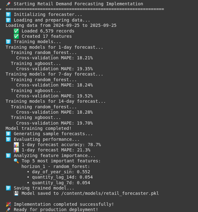
def main_implementation_example():

    """Full end-to-end instance"""

    print("🚀 Beginning Retail Demand Forecasting Implementation")

    print("=" * 60)

    # 1. Initialize forecaster

    print("1️⃣ Initializing forecaster...")

    forecaster = RetailDemandForecaster("connection_string_here")

    # 2. Load and put together information

    print("2️⃣ Loading and making ready information...")

    end_date = datetime.now().date()

    start_date = end_date - timedelta(days=365)

    raw_data = forecaster.load_and_prepare_data(start_date, end_date)

    processed_data = forecaster.create_advanced_features(raw_data)

    print(f"   ✅ Loaded {len(processed_data):,} data")

    print(f"   ✅ Created {len(processed_data.columns)} options")

    # 3. Practice fashions

    print("3️⃣ Coaching fashions...")

    forecaster.train_models(processed_data, forecast_horizons=[1, 7, 14])

    # 4. Make predictions on latest information

    print("4️⃣ Producing pattern forecasts...")

    recent_data = processed_data.tail(100)  # Final 100 data

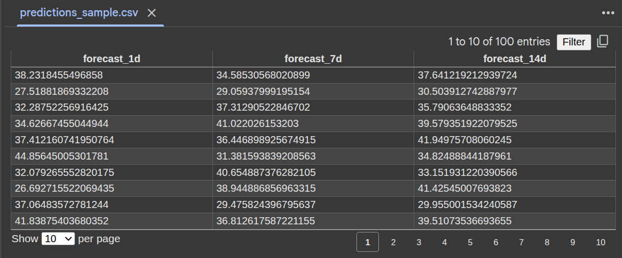
    predictions = forecaster.predict(recent_data, forecast_horizons=[1, 7, 14])

    # 5. Consider efficiency

    print("5️⃣ Evaluating efficiency...")

    # Create precise future values for analysis (simplified)

    actual_future = recent_data[['total_quantity']].copy()

    actual_future.columns = ['forecast_1d']  # Simplified analysis

    if 'forecast_1d' in predictions.columns:

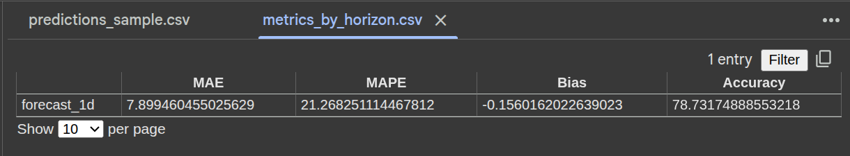
        metrics = forecaster.evaluate_performance(actual_future, predictions[['forecast_1d']])

        if metrics:

            print(f"   📊 1-day forecast accuracy: {metrics['forecast_1d']['Accuracy']:.1f}%")

            print(f"   📊 1-day forecast MAPE: {metrics['forecast_1d']['MAPE']:.1f}%")

    # 6. Analyze characteristic significance

    print("6️⃣ Analyzing characteristic significance...")

    significance = forecaster.analyze_feature_importance(top_n=5)

    if significance:

        print("   🔍 Prime 5 most vital options:")

        for horizon, fashions in significance.gadgets():

            for model_name, options in fashions.gadgets():

                print(f"      {horizon} - {model_name}:")

                for _, row in options.head(3).iterrows():

                    print(f"        • {row['feature']}: {row['importance']:.3f}")

                break  # Simply present one mannequin per horizon

            break  # Simply present one horizon

    # 7. Save mannequin

    print("7️⃣ Saving skilled mannequin...")

    import joblib

    joblib.dump(forecaster, 'fashions/retail_forecaster.pkl')

    print("   💾 Mannequin saved to fashions/retail_forecaster.pkl")

    print("n🎉 Implementation accomplished efficiently!")

    print("🚀 Prepared for manufacturing deployment!")

    return forecaster, predictions, metrics

# Run the instance

if __name__ == "__main__":

    forecaster, predictions, metrics = main_implementation_example()

Output:

Key Enterprise Advantages

Let’s quantify the price of the system implementation:

1. Stock Prices

• The Drawback: An excessive amount of stock creates prices related to capital {dollars} tied up and storage prices.
• The Answer: Use extra correct demand forecasts to scale back overstock by 15-25%
• The Influence: For a retailer with $100M of stock, this might save $3-6M a yr. 

2. Stockouts

• The Drawback: Empty cabinets imply misplaced gross sales and sad prospects.
• The Answer: Extra precisely predict demand and cut back stockouts by 20-30%
• The Influence: Recuperate 2-5% of income misplaced to stockouts. 

3. Operational Effectivity

• The Drawback: Guide processes for forecasting aren’t quick or dependable.
• The Answer: Automated programs can course of hundreds of SKUs in minutes.
• The Influence: Cut back the workload of your forecasting crew by 70%+.

Conclusion

Making a world-class demand forecasting system is each an artwork and a science. The science comes from the technical basis we now have created right here – superior characteristic engineering, ensemble machine studying, and production-ready deployment. The artwork comes from the information you perceive about your small business context and leveraging real-world efficiency to refine your demand forecast system regularly. 

The retail surroundings is changing into much more advanced; nonetheless, with an excellent forecasting system, you possibly can flip that complexity right into a aggressive benefit. Pleased forecasting!

Entry the total pocket book right here: Retail_Demand_Forecasting.ipynb

Ceaselessly Requested Questions

Knowledge Science Trainee at Analytics Vidhya
I’m at present working as a Knowledge Science Trainee at Analytics Vidhya, the place I concentrate on constructing data-driven options and making use of AI/ML methods to resolve real-world enterprise issues. My work permits me to discover superior analytics, machine studying, and AI functions that empower organizations to make smarter, evidence-based choices.
With a powerful basis in pc science, software program improvement, and information analytics, I’m obsessed with leveraging AI to create impactful, scalable options that bridge the hole between know-how and enterprise.
📩 You can even attain out to me at [email protected]