What’s KDE Plot? – Analytics Vidhya

Understanding the distribution of information is likely one of the most necessary elements of performing information evaluation. Visualizing the distribution helps us perceive the patterns, tendencies, and anomalies that could be hidden in uncooked numbers. Whereas histograms are sometimes used for this objective, they often might be too blocky to indicate some refined particulars. Kernel Density Estimation (KDE) plots present a smoother and extra correct method to visualize steady information by estimating its likelihood density operate. This permits information scientists and analysts to see necessary options akin to a number of peaks, skewness, and outliers extra clearly. Studying to make use of KDE plots is a helpful ability for higher understanding information insights. On this article, we’ll go over KDE plots and their implementations.

What are Kernel Density Estimation (KDE) Plots?

Kernel Density Estimation (KDE) is a non-parametric technique for estimating the likelihood density operate (PDF) of a steady random variable. Merely talking, KDE makes a clean curve (density estimate) which approximates the distribution of information, relatively than utilizing separated bins like in a histogram.  Idea-wise, we’ve a “kernel” (a clean and symmetric operate) on every information level and add them as much as type a steady density. Mathematically, if we’ve information factors x₁,…,x_n, then the KDE at a degree x is: 

The place Okay is the kernel (principally a bell form of operate) and h is the bandwidth (a smoothness parameter). Since no mounted type like “regular” or “exponential” is taken for the distribution, KDE is known as a non-parametric estimator. KDE “smooths a histogram” by turning every information level right into a small hill; all these hills collectively make the overall density (as might be seen from the next diagram).

Totally different sorts of kernel capabilities are used in keeping with the use case. For instance, the Gaussian (or regular) kernel is common due to its smoothness, however others like Epanechnikov (parabolic), uniform, triangular, biweight, and even triweight can be used. By default, many libraries go along with a Gaussian kernel, which means each information level provides a bell-shaped bump to the estimate. Epanechnikov kernel minimises the imply squared error between all, however nonetheless, the Gaussian is usually picked only for comfort.

Density plots are tremendous useful in analysing information to indicate the form of a distribution. They work properly for large datasets and might present issues (like a number of peaks or lengthy tails) {that a} histogram would possibly cover. For instance, KDE plots can catch bimodal or skewed shapes that let you know about sub-groups or outliers. When exploring a brand new numeric variable, plotting KDE is usually one of many first issues folks do. In some areas (like sign processing or econometrics), KDE can also be referred to as the Parzen-Rosenblatt window technique.

Necessary Ideas

Listed here are the important thing issues to remember when understanding how KDE plot works : 

• Non-parametric PDF estimation: KDE doesn’t assume the underlying distribution. It builds a clean estimate straight from the info.
• Kernel capabilities: A kernel Okay (e.g., Gaussian) is a symmetric weighting operate. Widespread selections embrace Gaussian, Epanechnikov, uniform, and so forth. The selection has a small impact on the end result so long as the bandwidth is adjusted.
• Bandwidth (smoothing): The parameter h (or, equivalently, bw ) scales the kernel. Bigger h yields smoother (wider) curves; smaller h yields tighter, extra detailed curves. The optimum bandwidth usually scales like n^−1/5.
• Bias-variance tradeoff: A key consideration is balancing element vs. smoothness: too small h results in a loud estimate; too massive h can oversmooth necessary peaks or valleys.

Utilizing KDE Plots in Python

Each Seaborn (constructed on Matplotlib) and pandas make it simple to create KDE plots in Python. Now, I will probably be displaying some utilization patterns, parameters, and customisation suggestions.

Seaborn’s kdeplot

First, use seaborn.kdeplot operate. This operate plots univariate (or bivariate) KDE curves for a dataset. Internally, it makes use of a Gaussian kernel by default and helps many different choices. For instance, to plot the distribution of the sepal_width variable from the Iris dataset.

Univariate KDE Plot Utilizing Seaborn (Iris Dataset Instance)

The next instance demonstrates how one can create a KDE plot for a single steady variable.

import seaborn as sns

import matplotlib.pyplot as plt

# Load instance dataset

df = sns.load_dataset('iris')

# Plot 1D KDE

sns.kdeplot(information=df, x='sepal_width', fill=True)

plt.title("KDE of Iris Sepal Width")

plt.xlabel("Sepal Width")

plt.ylabel("Density")

plt.present()

From the earlier picture, we are able to see a clean density curve of the speal_width values. Additionally, the fill=True argument shapes the realm underneath the curve, and whether it is fill = False, solely the darkish blue line would have been seen.

Evaluating KDE plots throughout Classes

Up to now, we’ve seen easy univariate KDE plots. Now, let’s see probably the most highly effective makes use of of Seaborn’s kdeplot technique, which is its capacity to check distributions throughout subgroups utilizing the hue parameter. 

Let’s say we need to analyse how the distribution of whole restaurant payments differs between lunch and dinner instances. So, for this, let’s use the suggestions dataset. With this, we are able to overlay two KDE plots, one for Lunch and one for Dinner, on the identical axes for direct comparability.

import seaborn as sns

import matplotlib.pyplot as plt

suggestions = sns.load_dataset('suggestions')

sns.kdeplot(information=suggestions, x='total_bill', hue="time", fill=True,

common_norm=False, alpha=0.5)

plt.title("KDE of Complete Invoice (Lunch vs Dinner)")

plt.present()

So we are able to see that the above code overlays two density curves. The fill=True shades underneath every curve to make the distinction extra seen, common_norm= False makes certain that every group’s density is scaled independently, and alpha=0.5 provides transparency so the overlapping areas are simple to interpret.

You may also experiment with a number of=‘layer’, ‘stack’, or ‘fill’ to alter how a number of densities are proven. 

Pandas and Matplotlib

If you’re working with pandas, you may also use built-in plotting to get KDE plots. A pandas collection has a plot(sort=’density’) or plot.density() technique that acts as a wrapper for the related strategies in Matplotlib.

Code:

import pandas as pd

import numpy as np

information = np.random.randn(1000) # 1000 random factors from a standard distribution

s = pd.Sequence(information)

s.plot(sort='density')

plt.title("Pandas Density Plot")

plt.xlabel("Worth")

plt.present()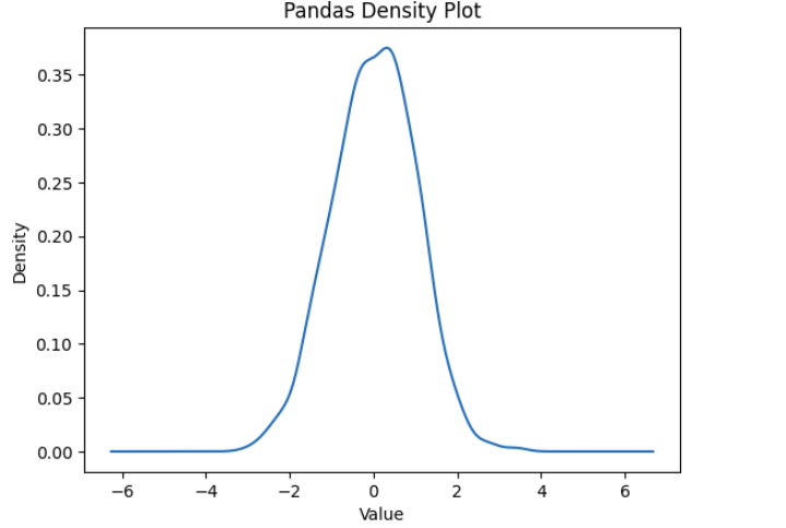

Alternatively, we are able to compute and plot KDE manually utilizing SciPy’s gaussian_kde technique.

import numpy as np

from scipy.stats import gaussian_kde

information = np.concatenate([np.random.normal(-2, 0.5, 300), np.random.normal(3,

1.0, 500)])

kde = gaussian_kde(information, bw_method=0.3) # bandwidth is usually a issue or

'silverman', 'scott'

xs = np.linspace(min(information), max(information), 200)

density = kde(xs)

plt.plot(xs, density)

plt.title("Handbook KDE by way of scipy")

plt.xlabel("Worth"); plt.ylabel("Density")

plt.present()

The above code creates a bimodal dataset and estimates its density. In follow, utilizing Seaborn or pandas for attaining the identical performance is way simpler. 

Deciphering KDE Plot or Kernel Density Estimator plot

Studying a KDE plot is much like a histogram, however with a clean curve. The peak of the curve at a degree x is proportional to the estimated likelihood density there. The realm underneath the curve over a spread corresponds to the likelihood of touchdown in that vary. As a result of the curve is steady, the precise worth at any level just isn’t as necessary as the general form:

• Peaks (modes): A excessive peak signifies a typical worth or cluster within the information. A number of peaks counsel a number of modes (e.g., combination of sub-populations).
• Unfold: The width of the curve exhibits dispersion. A wider curve means extra variability (bigger commonplace deviation), whereas a slim, tall curve means the info is tightly clustered.
• Tails: Observe how shortly the density tapers off. Heavy tails suggest outliers; quick tails suggest bounded information.
• Evaluating curves: When overlaying teams, search for shifts (one distribution systematically increased or decrease) or variations in form.

Use Circumstances and Examples

KDE plots have many helpful purposes in day-to-day information evaluation:

• Exploratory Information Evaluation (EDA): After we first have a look at a dataset, KDE helps us see how the variables are distributed, whether or not they look regular, skewed, or have a couple of peak(multimodal). As everyone knows that checking the distribution of your variables one after the other might be the primary job it is best to do while you get a brand new dataset. KDE, being smoother than histograms, is usually extra useful when attempting to get a really feel of the info throughout EDA.
• Evaluating distributions: KDE works properly after we need to examine how totally different teams behave. For instance, plotting the KDE of check scores for girls and boys on the identical axis exhibits if there’s any distinction in common or variation. Seaborn makes it tremendous simple to overlay KDE utilizing totally different colors. KDE plots are normally much less messy than side-by-side histograms, and so they give a greater sense of how the teams differ.
• Smoothing histograms: KDE might be considered a smoother model of a histogram. When histograms look too uneven or change quite a bit with bin dimension, KDE provides a extra steady and clear image. As an illustration, the Airbnb value instance above may very well be proven as a histogram, however KDE makes it a lot simpler to interpret. KDE helps create a extra steady estimate of the info’s form, which may be very helpful, particularly when the info isn’t too massive or too small.

Options to Kernel Density Plots

So, whereas KDE plots are tremendous helpful for displaying clean estimates of a distribution, they don’t seem to be all the time the most effective factor to make use of. Relying on the info dimension or what precisely you are attempting to do, there are different sorts of plots you may strive, too. Listed here are a couple of frequent ones:

Histograms

Actually, essentially the most primary means to take a look at distributions. You simply chop the info into bins and rely what number of issues fall in every. Simple to make use of, however can get messy for those who use too many bins or too few. Typically it hides patterns. KDE form of helps with that by smoothing the bumps.

Field Plots(additionally referred to as box-and-whisker)

These are good for those who simply wanna know, like the place many of the information is, you get the median, quartiles, and so forth. It’s quick to identify outliers. Nevertheless it doesn’t actually present the form of the info like KDE does. Nonetheless helpful while you don’t want each element.

Violin Plots

Consider these like a flowery model of field plots that additionally exhibits the KDE form. It’s like the most effective of each, you get abstract stats and a way of distribution. I take advantage of these when evaluating teams facet by facet.

Rug Plots

Rug plots are easy. They only present every information level as small vertical traces on the axis. Typically, together with KDE, to indicate the place the true information factors are. However when you’ve an excessive amount of information, it might look form of messy.

Histogram + KDE Combo

Some folks like to mix a histogram with KDE, as a histogram exhibits the counts and KDE provides a clean curve on prime. This manner, they will see each uncooked frequencies and the smoothed sample collectively. 

Actually, which one you utilize simply relies on what you want. KDE is nice for clean patterns, however typically you don’t want all that; possibly a easy field plot or histogram says sufficient, particularly if you’re quick on time or simply exploring stuff shortly.

Conclusion

KDE plots provide a robust and intuitive method to visualize the distribution of steady information. In contrast to regular histograms, they offer a clean and steady curve by estimating the likelihood density operate with the assistance of kernels, which makes refined patterns like skewness, multimodality, or outliers simpler to note. Whether or not you’re doing Exploratory Information Evaluation, evaluating distributions, or discovering anomalies, KDE plots are actually useful. Instruments like Seaborn or pandas make it fairly easy to create and use them.

Hello, I’m Janvi, a passionate information science fanatic at present working at Analytics Vidhya. My journey into the world of information started with a deep curiosity about how we are able to extract significant insights from advanced datasets.