Methods to Use Python Pandas and SQL Collectively for Information Evaluation

For all of the duties associated to knowledge science and machine studying, crucial factor that defines how a mannequin will carry out relies on how good our knowledge is. Python Pandas and SQL are among the many highly effective instruments that may assist in extracting and manipulating knowledge effectively. By combining these two collectively, knowledge analysts can carry out complicated evaluation on even massive datasets. On this article, we’ll discover how one can mix Python Pandas with SQL to boost the standard of information evaluation.

Pandas and SQL: Overview

Earlier than utilizing Pandas and SQL collectively. First, we’ll undergo Pandas and SQL is able to and their key options.

What’s Pandas?

Pandas is a software program library written for Python programming language for knowledge manipulation and evaluation. It provides operations for manipulating tables, knowledge constructions, and time collection knowledge.

Key Options of Pandas

• Pandas DataFrames enable us to work with structured knowledge. 
• It provides completely different functionalities like sorting, grouping, merging, reshaping, and filtering knowledge.
• It’s environment friendly in dealing with lacking knowledge values.

Study Extra: The Final Information to Pandas For Information Science!

What’s SQL?

SQL stands for Structured Question Language, which is used for extracting, managing, and manipulating relational databases. It’s helpful in dealing with structured knowledge by incorporating relations amongst entities and variables. It permits for inserting, updating, deleting, and managing the saved knowledge in tables. 

Key Options of SQL

• It supplies a sturdy method for querying massive datasets.
• It permits the creation, modification, and deletion of database schemas.
• The syntax of SQL is optimized for environment friendly and sophisticated question operations like JOIN, GROUPBY, ORDER BY, HAVING, utilizing sub-queries.

Study Extra: SQL For Information Science: A Newbie’s Information!

Why Mix Pandas with SQL?

Utilizing Pandas and SQL collectively makes the code extra readable and, in sure circumstances, simpler to implement. That is true for complicated workflows, as SQL queries are a lot clearer and simpler to learn than the equal Pandas code. Furthermore, many of the relational knowledge originates from databases, and SQL is likely one of the foremost instruments to take care of relational knowledge. This is likely one of the foremost explanation why working professionals like knowledge analysts and knowledge scientists desire to combine their functionalities.

How Does pandasql Work?

To mix SQL queries with Pandas, one wants a standard bridge between these two, so to beat this downside, ‘pandasql’ comes into the image. Pandasql lets you run SQL queries instantly inside Pandas. On this method, we are able to seamlessly use the SQL syntax with out leaving the dynamic Pandas setting.

Putting in pandasql

Step one to utilizing Pandas and SQL collectively is to put in pandasql into our surroundings.

pip set up pandasql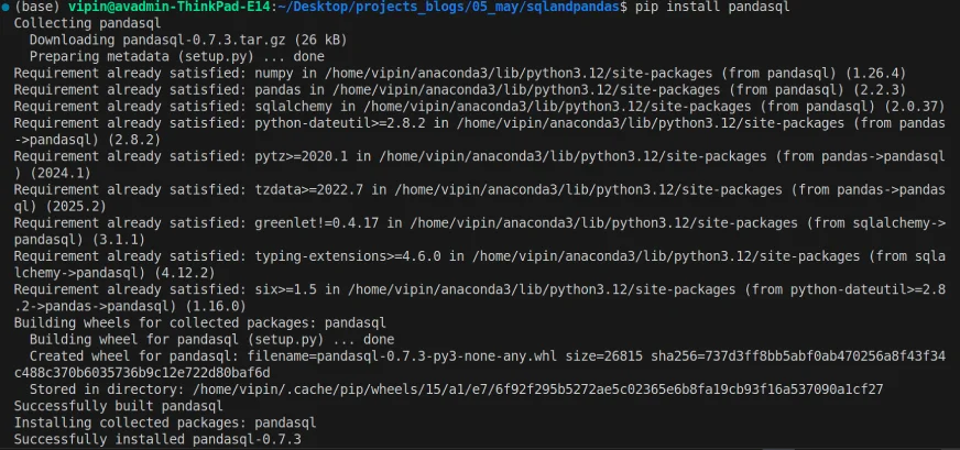

As soon as the set up is full, we are able to import the pandasql into our code and use it to execute the SQL queries on Pandas DataFrame.

Working SQL Queries in Pandas

As soon as the set up is over, we are able to import the pandasql and begin exploring it.

import pandas as pd
import pandasql as psql

# Create a pattern DataFrame
knowledge = {'Identify': ['Alice', 'Bob', 'Charlie'], 'Age': [25, 30, 35]}
df = pd.DataFrame(knowledge)

# SQL question to pick all knowledge
question = "SELECT * FROM df"
consequence = psql.sqldf(question, locals())
consequence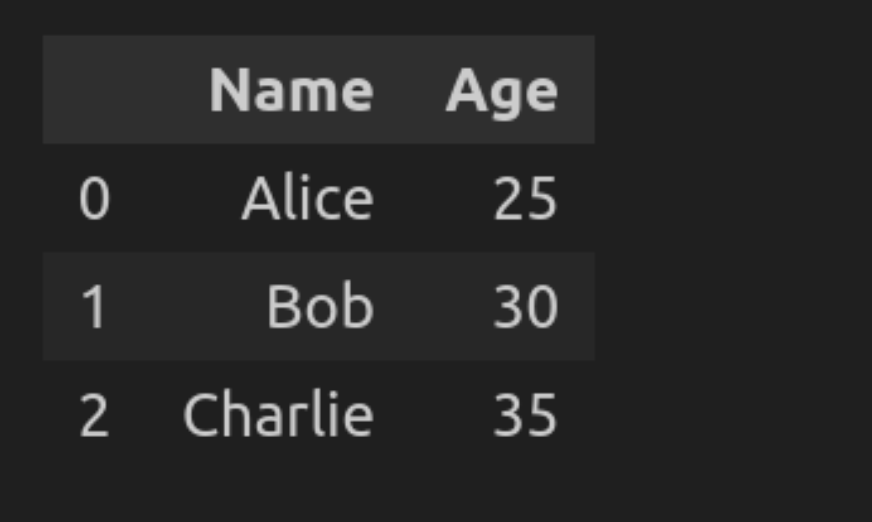

Let’s break down the code

• pd.DataFrame will convert the pattern knowledge right into a tabular format.
• question (SELECT * FROM df) will choose every little thing within the type of the DataFrame. 
• psql.sqldf(question, locals()) will execute the SQL question on the DataFrame utilizing the native scope.

Information Evaluation with pandasql

As soon as all of the libraries are imported, it’s time to carry out the information evaluation utilizing pandasql. The beneath part exhibits just a few examples of how one can improve the information evaluation by combining Pandas and SQL. To do that:

Step 1: Load the Information

# Required libraries
import pandas as pd
import pandasql as ps
import plotly.specific as px
import ipywidgets as widgets
# Load the dataset
car_data = pd.read_csv("cars_datasets.csv")
car_data.head()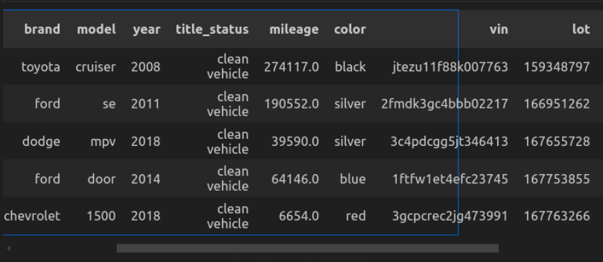

Let’s break down the code

• Importing the mandatory libraries: pandas for dealing with knowledge, pandasql for querying the DataFrames, plotly for making interactive plots.
• pd.read_csv(“cars_datasets.csv”) to load the information from the native listing.
• car_data.head() will show the highest 5 rows.

Step 2: Discover the Information

On this part, we’ll attempt to get aware of knowledge by exploring issues just like the names of columns, the information kind of the options, and whether or not the information has any null values or not.

1. Test the column names.

# Show column names
column_names = car_data.columns
column_names
"""
Output:
Index(['Unnamed: 0', 'price', 'brand', 'model', 'year', 'title_status',
      'mileage', 'color', 'vin', 'lot', 'state', 'country', 'condition'],
     dtype="object")
""”

2. Determine the information kind of the columns.

# Show dataset information
car_data.information()
"""
Ouput:

RangeIndex: 2499 entries, 0 to 2498
Information columns (whole 13 columns):
#   Column        Non-Null Depend  Dtype 
---  ------        --------------  ----- 
0   Unnamed: 0    2499 non-null   int64 
1   value         2499 non-null   int64 
2   model         2499 non-null   object
3   mannequin         2499 non-null   object
4   12 months          2499 non-null   int64 
5   title_status  2499 non-null   object
6   mileage       2499 non-null   float64
7   coloration         2499 non-null   object
8   vin           2499 non-null   object
9   lot           2499 non-null   int64 
10  state         2499 non-null   object
11  nation       2499 non-null   object
12  situation     2499 non-null   object
dtypes: float64(1), int64(4), object(8)
reminiscence utilization: 253.9+ KB
"""

3. Test for Null values.

# Test for null values
car_data.isnull().sum()


"""Output:
Unnamed: 0      0
value           0
model           0
mannequin           0
12 months            0
title_status    0
mileage         0
coloration           0
vin             0
lot             0
state           0
nation         0
situation       0
dtype: int64
"""

Step 3: Analyze the Information

As soon as we’ve got loaded the dataset into the workflow. Now we are going to start by performing knowledge evaluation.

Examples of Information Evaluation with Python Pandas and SQL

Now let’s attempt utilizing pandasql to investigate the above dataset by operating a few of our queries.

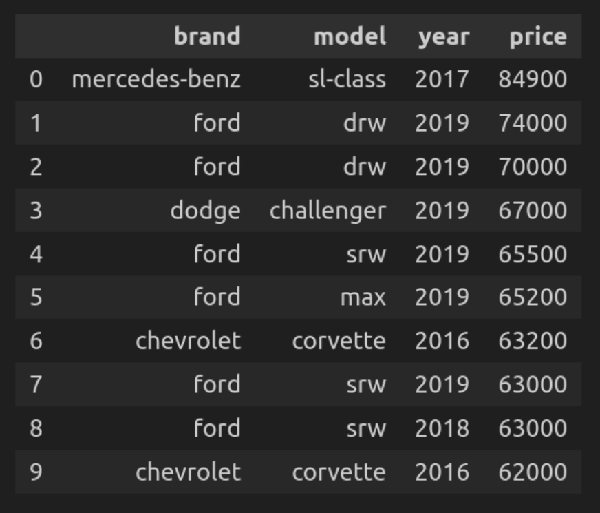
Question 1: Deciding on the ten Most Costly Automobiles

Let’s first discover the highest 10 most costly automobiles from the whole dataset.

def q(question):
   return ps.sqldf(question, {'car_data': car_data})
q("""
SELECT model, mannequin, 12 months, value
FROM car_data
ORDER BY value DESC
LIMIT 10
""")

Let’s break down the code

• q(question) is a customized operate that executes the SQL question on the DataFrame.
• The question iterates over the entire dataset and selects columns corresponding to model, mannequin, 12 months, value, after which types them by value in descending order.

Question 2: Common Worth by Model

Right here we’ll discover the common value of automobiles for every model.

def q(question):
   return ps.sqldf(question, {'car_data': car_data})

q("""
SELECT model, ROUND(AVG(value), 2) AS avg_price
FROM car_data
GROUP BY model
ORDER BY avg_price DESC""")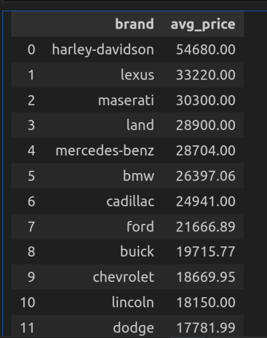

Let’s break down the code

• Right here, the question makes use of AVG(value) to calculate the common value for every model and makes use of spherical, spherical off the resultant to 2 decimals.
• And GROUPBY will group the information by the automotive manufacturers and type it through the use of the AVG(value) in descending order.

Question 3: Automobiles Manufactured After 2015

Let’s make a listing of the automobiles manufactured after 2015.

def q(question):
   return ps.sqldf(question, {'car_data': car_data})

q("""
SELECT *
FROM car_data
WHERE 12 months > 2015
ORDER BY 12 months DESC
""")

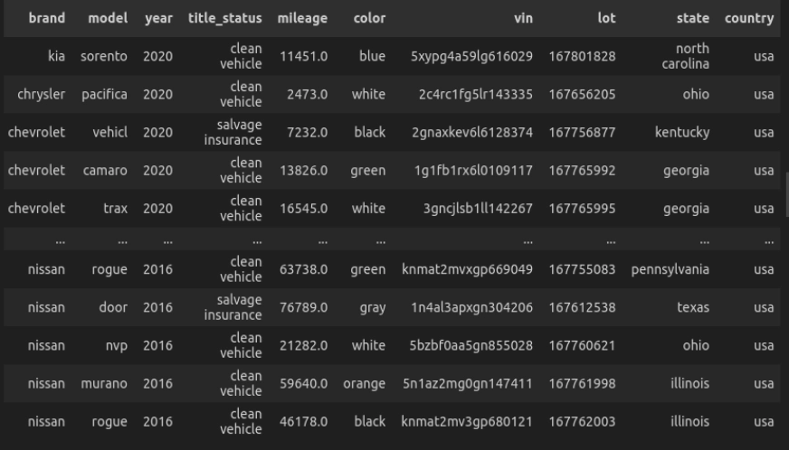
Let’s break down the code

• Right here, the question selects all of the automotive producers after 2015 and orders them in descending order.

Question 4: High 5 Manufacturers by Variety of Automobiles Listed

Now let’s discover the entire variety of automobiles produced by every model.

def q(question):
   return ps.sqldf(question, {'car_data': car_data})

q("""
SELECT model, COUNT(*) as total_listed
FROM car_data
GROUP BY model
ORDER BY total_listed DESC
LIMIT 5
""")

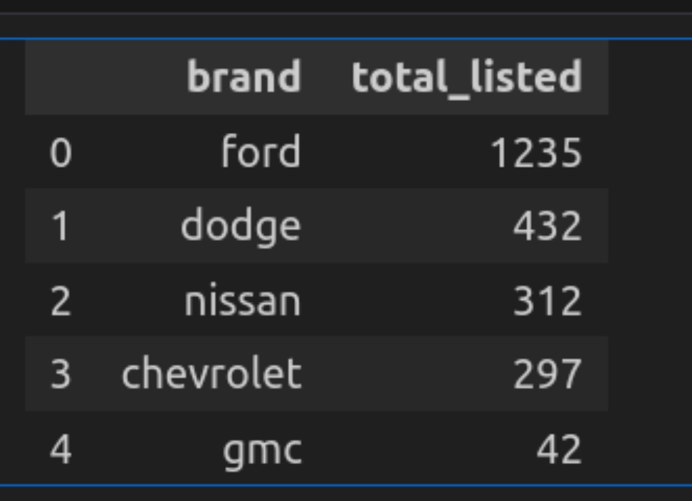
Let’s break down the code

• Right here the question counts the entire variety of automobiles by every model utilizing the GROUP BY operation.
• It lists them in descending order and makes use of a restrict of 5 to pick solely the highest 5.

Question 5: Common Worth by Situation

Let’s see how we are able to group the automobiles primarily based on a situation. Right here, the situation column exhibits the time when the itemizing was added or how a lot time is left. Primarily based on that, we are able to categorize the automobiles and get their common pricing.

def q(question):
   return ps.sqldf(question, {'car_data': car_data})

q("""
SELECT situation, ROUND(AVG(value), 2) AS avg_price, COUNT(*) as listings
FROM car_data
GROUP BY situation
ORDER BY avg_price DESC
""")

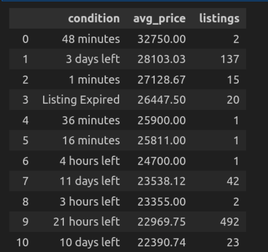
Let’s break down the code

• Right here, the question teams the automobiles on situation (corresponding to new or used) and calculates the value utilizing AVG(Worth).
• Get them organized in descending order to point out the most costly automobiles first.

Question 6: Common Mileage and Worth by Model

Right here we’ll discover the common mileage of the automobiles for every model and their common value. 

def q(question):
   return ps.sqldf(question, {'car_data': car_data})

q("""
SELECT model,
      ROUND(AVG(mileage), 2) AS avg_mileage,
      ROUND(AVG(value), 2) AS avg_price,
      COUNT(*) AS total_listings
FROM car_data
GROUP BY model
ORDER BY avg_price DESC
LIMIT 10
""")

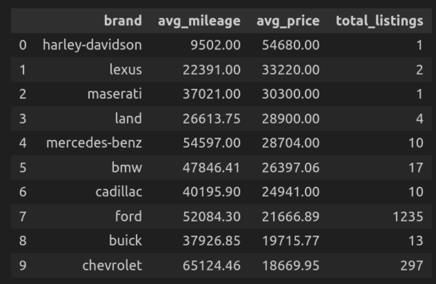
Let’s break down the code

• Right here, the question teams the automobiles utilizing model and calculates their common mileage and common value, and counts the entire variety of listings of every model in that group.
• Get them organized in descending order by value.

Question 7: Worth per Mileage Ratio for High Manufacturers

Now let’s kind the highest manufacturers primarily based on their calculated mileage ratio i.e. the common value per mile of the automobiles for every model.

def q(question):
   return ps.sqldf(question, {'car_data': car_data})

q("""
SELECT model,
      ROUND(AVG(value/mileage), 4) AS price_per_mile,
      COUNT(*) AS whole
FROM car_data
WHERE mileage > 0
GROUP BY model
ORDER BY price_per_mile DESC
LIMIT 10
""")

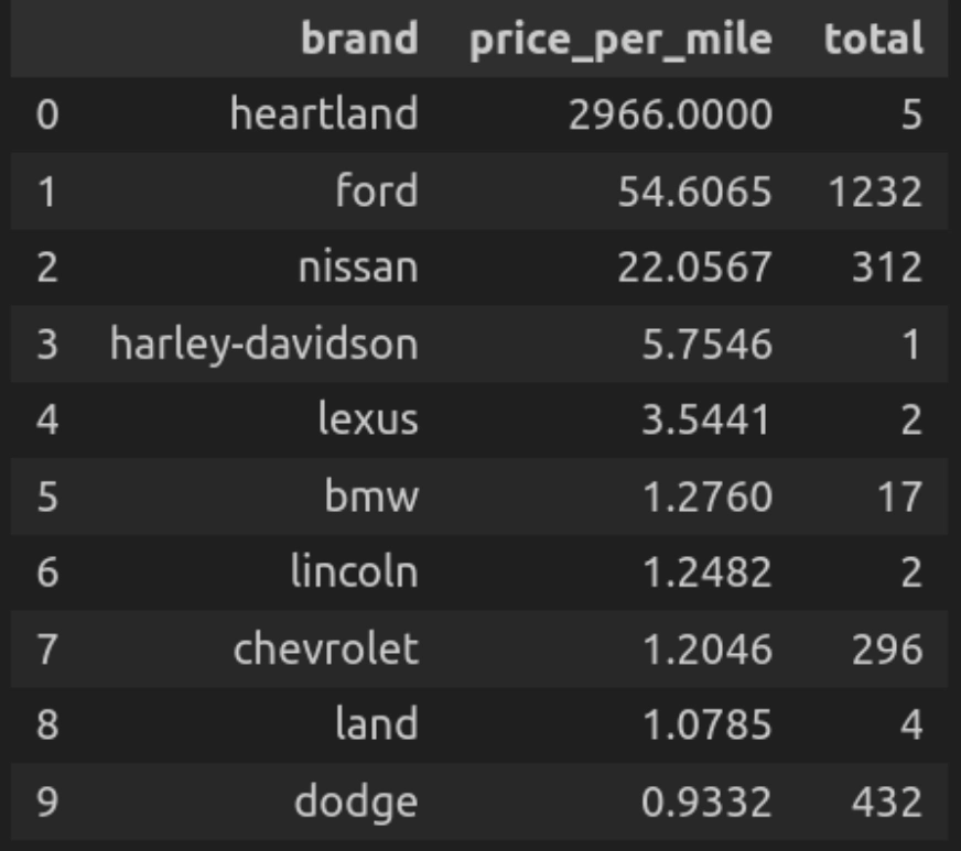
Let’s break down the code

• Right here question calculates the value per mileage for every model after which exhibits automobiles by every model with that particular value per mileage. In descending order by value per mile.

Question 8: Common Automotive Worth by Space

Right here we’ll discover and plot the variety of automobiles of every model in a selected metropolis. 

state_dropdown = widgets.Dropdown(
   choices=car_data['state'].distinctive().tolist(),
   worth=car_data['state'].distinctive()[0],
   description='Choose State:',
   format=widgets.Format(width="50%")
)

def plot_avg_price_state(state_selected):
   question = f"""
       SELECT model, AVG(value) AS avg_price
       FROM car_data
       WHERE state="{state_selected}"
       GROUP BY model
       ORDER BY avg_price DESC
   """
   consequence = q(question)
   fig = px.bar(consequence, x='model', y='avg_price', coloration="model",
                title=f"Common Automotive Worth in {state_selected}")
   fig.present()

widgets.work together(plot_avg_price_state, state_selected=state_dropdown)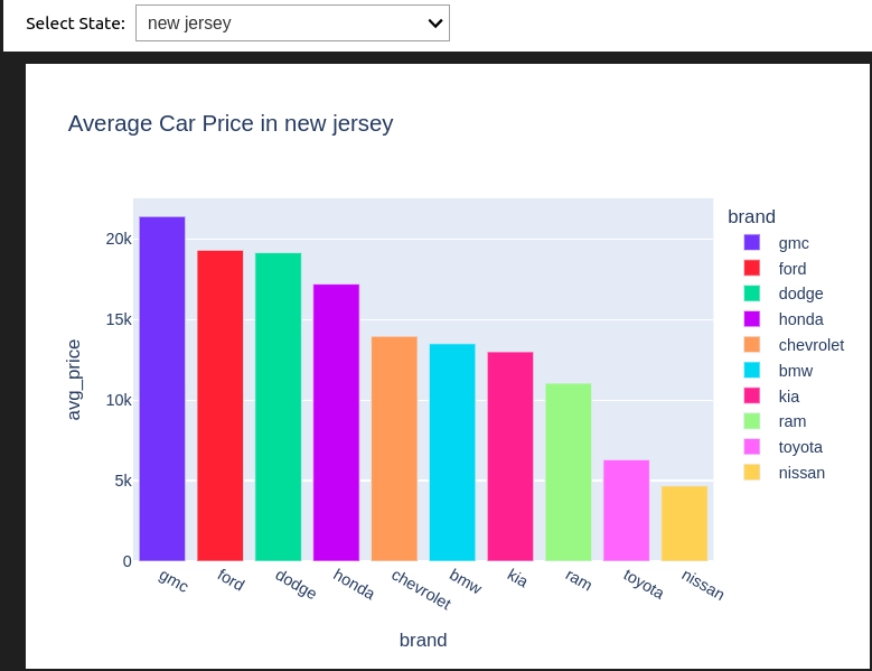

Let’s break down the code

• State_dropdown creates a dropdown to pick the completely different US states from the information and permits the person to pick a state.
• plot_avg_price_state(state_selected) executes the question to calculate the common value per model and provides a bar chart utilizing plotly.
• widgets.work together() hyperlinks the dropdown with the operate so the chart can replace by itself when the person selects a special state.

For the pocket book and the dataset used right here, please go to this hyperlink.

Limitations of pandasql

Regardless that pandasql provides many environment friendly functionalities and a handy option to run SQL queries with Pandas, it additionally has some limitations. On this part, we’ll discover these limitations and take a look at to determine when to depend on conventional Pandas or SQL, and when to make use of pandasql.

• Not suitable with massive datasets: Whereas we run the pandasql question creates a replica of the information in reminiscence earlier than full execution of the present question. This methodology of executing the over queries coping with massive datasets can result in excessive reminiscence utilization and sluggish execution.
• Restricted SQL Options:  pandasql helps many fundamental SQL options, but it surely fails to completely implement all of the superior options like subqueries, complicated joins, and window capabilities.
• Compatibility with Advanced Information: pandas works nicely with tabular knowledge. Whereas working with complicated knowledge, corresponding to nested JSON or multi-index DataFrames, it fails to offer the specified outcomes.

Conclusion

Utilizing Pandas and SQL collectively considerably improves the information evaluation workflow. By leveraging pandasql, one can seamlessly run SQL queries within the DataFrames. This helps those that are aware of SQL and need to work in Python environments. This integration of Pandas and SQL combines the flexibleness of each and opens up new prospects for knowledge manipulation and evaluation. With this, one can improve the power to sort out a variety of information challenges. Nonetheless, it’s necessary to think about the constraints of pandasql as nicely, and discover different approaches when coping with massive and sophisticated datasets.

Good day! I am Vipin, a passionate knowledge science and machine studying fanatic with a robust basis in knowledge evaluation, machine studying algorithms, and programming. I’ve hands-on expertise in constructing fashions, managing messy knowledge, and fixing real-world issues. My purpose is to use data-driven insights to create sensible options that drive outcomes. I am desperate to contribute my expertise in a collaborative setting whereas persevering with to be taught and develop within the fields of Information Science, Machine Studying, and NLP.