4 LLM Compression Methods That You Cannot Miss

LLMs like these from Google and OpenAI have proven unimaginable talents. However their energy comes at a value. These large fashions are sluggish, costly to run, and troublesome to deploy on on a regular basis gadgets. That is the place LLM compression methods are available. These strategies shrink fashions, making them sooner and extra accessible and not using a main loss in efficiency. This information explores 4 key methods: mannequin quantization, mannequin pruning strategies, data distillation in LLMs, and Low-Rank Adaptation (LoRA), full with hands-on code examples.

Why Do We Want LLM Compression?

Earlier than diving into the “how,” let’s perceive the “why.” Compressing LLMs affords clear benefits that make them sensible for real-world use.

• Lowered Mannequin Measurement: Smaller fashions require much less storage, making them simpler to host and distribute.
• Quicker Inference: A compact mannequin can generate responses extra shortly. This improves the person expertise in functions like chatbots.
• Decrease Prices: Lowered dimension and sooner pace result in decrease wants for reminiscence and processing energy. This cuts down on cloud computing and power prices.
• Better Accessibility: Compression permits highly effective fashions to run on gadgets with restricted sources, like smartphones and laptops.

Method 1: Quantization – Doing Extra with Much less

Mannequin quantization is without doubt one of the hottest and efficient LLM compression methods. It really works by decreasing the precision of the numbers (weights) that make up the mannequin. Consider it like saving a high-resolution photograph as a compressed JPEG; you lose a tiny quantity of element, however the file dimension shrinks dramatically. Most fashions are skilled utilizing 32-bit floating-point numbers (FP32). Quantization converts these to smaller 8-bit integers (INT8) and even 4-bit integers.

This picture visually explains quantization, the place steady, high-precision FP32 (32-bit floating-point) values are mapped to a restricted set of discrete, lower-precision INT4 (4-bit integer) values. Primarily, it reveals how a variety of floating-point numbers are approximated by a smaller, mounted variety of integer ranges to scale back reminiscence and computation, although this may introduce some precision loss.

Arms-On: 4-bit Quantization with Hugging Face

Let’s quantize a mannequin utilizing the Hugging Face transformers and bitsandbytes library. This instance reveals the right way to load a mannequin in 4-bit precision, considerably decreasing its reminiscence footprint.

Step 1: Set up Libraries
First, guarantee you could have the required libraries put in.

!pip set up transformers torch speed up bitsandbytes -q

Step 2: Load and Examine Fashions
We are going to load a normal mannequin after which its quantized model to see the distinction.

import torch

from transformers import AutoModelForCausalLM, AutoTokenizer

# We use a smaller, well-known mannequin for this demonstration

model_id = "gpt2"

print(f"Loading tokenizer for mannequin: {model_id}")

tokenizer = AutoTokenizer.from_pretrained(model_id)

print("n-----------------------------------")

print("Loading unique mannequin in FP32...")

# Load the unique mannequin in full precision (Float32)

model_fp32 = AutoModelForCausalLM.from_pretrained(model_id)

# Test the reminiscence footprint of the unique mannequin

print("nOriginal mannequin reminiscence footprint:")

# Calculate reminiscence footprint manually

mem_fp32 = sum(p.numel() * p.element_size() for p in model_fp32.parameters())

print(f"{mem_fp32 / 1024**2:.2f} MB")

print("n-----------------------------------")

print("Loading mannequin with 4-bit quantization...")

# Load the identical mannequin with 4-bit quantization enabled

model_4bit = AutoModelForCausalLM.from_pretrained(

   model_id,

   load_in_4bit=True,

   device_map="auto" # Routinely makes use of the GPU if out there

)

# Test the reminiscence footprint of the 4-bit mannequin

print("n4-bit quantized mannequin reminiscence footprint:")

# Calculate reminiscence footprint manually

mem_4bit = sum(p.numel() * p.element_size() for p in model_4bit.parameters())

print(f"{mem_4bit / 1024**2:.2f} MB")

print("nNotice the numerous discount in reminiscence utilization!")

Output:

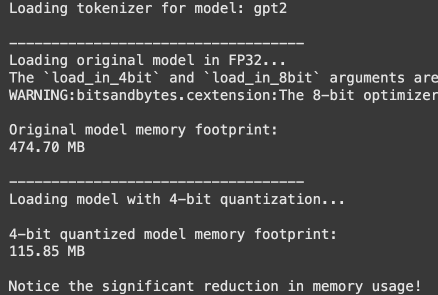
You’ll discover a big discount within the mannequin’s reminiscence utilization with virtually no change to the standard of its output for many duties.

Method 2: Pruning – Trimming Away Unused Connections

Mannequin pruning strategies work by eradicating elements of the neural community that contribute the least to its output. It’s like trimming a plant to encourage more healthy progress. You possibly can take away particular person weights (unstructured pruning) or whole teams of neurons (structured pruning). Whereas highly effective, pruning might be advanced to implement appropriately.

Unstructured pruning, for example, removes particular person weights based mostly on their magnitude, making a sparse mannequin. Whereas this makes the mannequin smaller, it may be troublesome for {hardware} to reap the benefits of the sparse construction. Structured pruning removes whole blocks, like neurons or layers, which is usually extra hardware-friendly.

The picture illustrates totally different methods for pruning elements just like the Imaginative and prescient Transformer (ViT) and the Giant Language Mannequin (LLM) utilizing “pruning layers” to scale back mannequin dimension and enhance effectivity. Particularly, (a) reveals pruning within the visible encoder, (b) focuses on pruning throughout the LLM, and (c) introduces an “instruction-guided part” to dynamically prune visible tokens based mostly on textual directions, enhancing effectivity for duties like video understanding.

Method 3: Information Distillation – The Pupil-Instructor Method

Information distillation in LLMs is a captivating course of. A big, extremely correct “instructor” mannequin trains a smaller “scholar” mannequin. The coed learns to imitate the instructor’s thought course of (its output chances), not simply the ultimate reply. This permits the smaller mannequin to realize efficiency far past what it may by coaching on the information alone.

This picture illustrates three data distillation strategies in machine studying: offline, on-line, and self-distillation. Offline distillation makes use of a pre-trained “instructor” to coach a “scholar”, whereas on-line distillation trains each concurrently, and self-distillation includes a single mannequin performing as each instructor and scholar (e.g., deeper layers educating shallower ones). The orange “instructor” fashions are pre-trained, whereas the blue “scholar” fashions (together with the mixed “instructor/scholar” in self-distillation) are “to be skilled”. 

Arms-On: Conceptual Distillation with Hugging Face

Implementing a full distillation pipeline is concerned, however the core thought might be understood via the Hugging Face Coach API.

from transformers import TrainingArguments, Coach

# This can be a conceptual instance as an example the method.

# To run this, you would want:

# 1. An outlined 'teacher_model' (a big, pre-trained mannequin).

# 2. An outlined 'student_model' (a smaller mannequin to be skilled).

# 3. A 'your_dataset' object for coaching.

# Outline Coaching Arguments

training_args = TrainingArguments(

   output_dir="./student_model_distilled",

   num_train_epochs=1, # Instance worth

   per_device_train_batch_size=8, # Instance worth

   # ... different coaching arguments

)

# Create a customized Coach to change the loss perform

class DistillationTrainer(Coach):

   def compute_loss(self, mannequin, inputs, return_outputs=False):

       # That is the core of information distillation.

       # The loss perform is a weighted common of two elements:

       #   a) The coed's commonplace loss on the information (e.g., Cross-Entropy).

       #   b) The distillation loss, which measures how nicely the scholar's

       #      output distribution matches the instructor's.

       # This half is conceptual and requires a full implementation.

       print("Inside customized compute_loss - that is the place distillation logic would go.")

       # For instance:

       # student_outputs = mannequin(**inputs)

       # student_loss = student_outputs.loss

       # with torch.no_grad():

       #     teacher_outputs = teacher_model(**inputs)

       # distillation_loss = some_kl_divergence_loss(student_outputs.logits, teacher_outputs.logits)

       # combined_loss = 0.5 * student_loss + 0.5 * distillation_loss

       # Returning a dummy loss to stop errors on this conceptual instance

       dummy_outputs = mannequin(**inputs)

       return (dummy_outputs.loss, dummy_outputs) if return_outputs else dummy_outputs.loss

print("The DistillationTrainer class is outlined conceptually.")

print("A full implementation would require a instructor mannequin, scholar mannequin, and a dataset.")

This course of successfully transfers the “data” from the big mannequin to the smaller one.

Method 4: Low-Rank Adaptation (LoRA) – Environment friendly Positive-Tuning

Whereas not a technique to shrink a base mannequin, Low-Rank Adaptation (LoRA) is a method to compress the adjustments made throughout fine-tuning. As an alternative of retraining all of the billions of parameters in a mannequin, LoRA freezes the unique mannequin and injects tiny, trainable “adapter” layers. These adapters are a lot smaller, making the fine-tuning course of sooner and the ensuing fine-tuned mannequin way more memory-efficient to retailer and swap between.

This diagram explains LoRA (Low-Rank Adaptation) for environment friendly mannequin fine-tuning: throughout coaching, a small, trainable low-rank adaptation matrix (BA) is added to the frozen pretrained weights (W). After coaching, this low-rank matrix is merged with the unique weights, successfully making a specialised mannequin (W + BA) with out rising inference latency or reminiscence footprint throughout deployment. This considerably reduces computational sources and storage necessities in comparison with full fine-tuning.

Arms-On: Positive-Tuning with LoRA and PEFT

The Hugging Face PEFT (Parameter-Environment friendly Positive-Tuning) library makes making use of LoRA easy.

Step 1: Set up Libraries

!pip set up peft -q 

Step 2: Apply LoRA and Examine Parameter Counts

from peft import get_peft_model, LoraConfig, TaskType

from transformers import AutoModelForCausalLM

model_id = "gpt2"

mannequin = AutoModelForCausalLM.from_pretrained(model_id)

# Outline the LoRA configuration

lora_config = LoraConfig(

   task_type=TaskType.CAUSAL_LM, # Specify the duty sort

   r=8,  # Rank of the replace matrices. Decrease rank means fewer parameters.

   lora_alpha=32, # A scaling issue for the discovered weights.

   lora_dropout=0.1, # Dropout chance for LoRA layers.

   target_modules=["c_attn"] # Apply LoRA to the eye layers of GPT-2.

)

# Wrap the bottom mannequin with the LoRA adapters

lora_model = get_peft_model(mannequin, lora_config)

print("--- Authentic Mannequin ---")

# Get the whole variety of parameters for the unique mannequin

total_params = sum(p.numel() for p in mannequin.parameters())

print(f"Complete parameters: {total_params:,}")

print("n--- LoRA Tailored Mannequin ---")

# The PeftModel object has the print_trainable_parameters technique

lora_model.print_trainable_parameters()

print("nNote how LoRA reduces trainable parameters by over 99%!")

print("This makes fine-tuning way more environment friendly.")

Output:

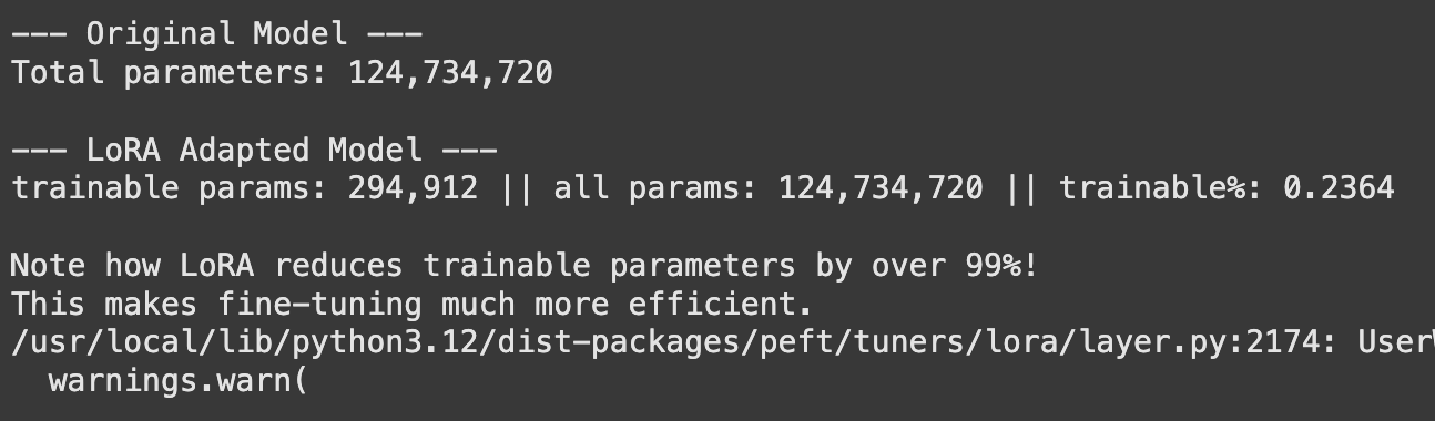
The output will present a dramatic discount (usually over 99%) within the variety of parameters that have to be skilled and saved. This makes it doable to fine-tune and handle many alternative variations of a mannequin for numerous duties with out storing enormous mannequin recordsdata for each.

You’ll find the total Colab pocket book right here: Colab

Conclusion

Giant Language Fashions are right here to remain, however their large dimension presents an actual problem. LLM compression methods are the important thing to unlocking their potential for a wider vary of functions. Whether or not it’s the simple method of mannequin quantization, the surgical precision of mannequin pruning strategies, the intelligent mentorship of information distillation in LLMs, or the effectivity of Low-Rank Adaptation (LoRA), these strategies make AI extra sensible. The proper method is determined by your particular wants, however combining them can usually result in the perfect outcomes.

Often Requested Questions

Harsh Mishra is an AI/ML Engineer who spends extra time speaking to Giant Language Fashions than precise people. Captivated with GenAI, NLP, and making machines smarter (so that they don’t change him simply but). When not optimizing fashions, he’s in all probability optimizing his espresso consumption. 🚀☕